Date/Time Features

​

Why incorporate Date/Time Features in your Forecasts

Many time series display patterns that repeat based on the calendar like demand increasing on weekends, sales peaking at the end of the month, or traffic varying by hour of the day. Recognizing and capturing these time-based patterns can be a powerful way to improve forecasting accuracy.

While you can forecast a time series based solely on its historical values, adding additional date/time related features, such as the day of the week, month, quarter, or hour, can often enhance the model’s performance. These features can be especially useful when your dataset lacks exogenous variables, but they can also complement external regressors when available.

In this tutorial, we’ll walk through how to incorporate these date/time features into TimeGPT to boost the accuracy of your forecasts.

​

How to incorporate Date/Time Features in your Forecasts

​

Step 1: Import Packages

Import the necessary libraries and initialize the Nixtla client.

import numpy as np
import pandas as pd
from nixtla import NixtlaClient

# For forecast evaluation
from utilsforecast.evaluation import evaluate
from utilsforecast.losses import mae, rmse

You can instantiate the NixtlaClient class providing your authentication API key.

nixtla_client = NixtlaClient(
    # defaults to os.environ.get("NIXTLA_API_KEY")
    api_key='my_api_key_provided_by_nixtla'
)

​

Step 2: Load Data

In this notebook, we use hourly electricity prices as our example dataset, which consists of 5 time series, each with approximately 1700 data points. For demonstration purposes, we focus on the German electricity price series. The time series is split, with the last 240 steps (10 days) set aside as the test set.

For simplicity, we will also demonstrate this tutorial without the use of any additional exogenous variables, but you could extend this same technique for datasets that have exogenous variables.

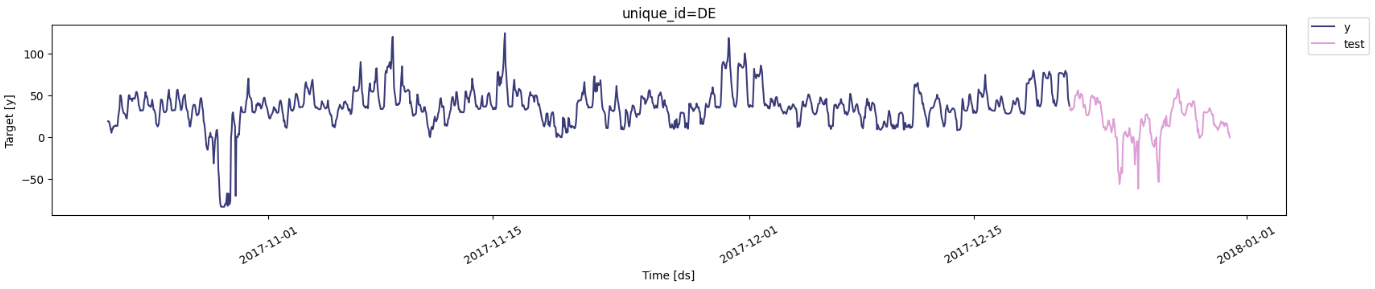
df = pd.read_csv(
    'https://raw.githubusercontent.com/Nixtla/transfer-learning-time-series/main/datasets/electricity-short-with-ex-vars.csv'
)
df['ds'] = pd.to_datetime(df['ds'])
df_sub = df.query('unique_id == "DE"')[['unique_id','ds','y']]

df_train = df_sub.query('ds < "2017-12-21"')
df_test = df_sub.query('ds >= "2017-12-21"')
df_train.shape, df_test.shape

((1440, 3), (240, 3))

nixtla_client.plot(df_train, df_test.rename(columns={'y': 'test'}))

​

Step 3: Forecasting

​

Without Datetime Features

First, we forecast the univariate time series without the use of datetime features.

fcst_timegpt_no_dt = nixtla_client.forecast(
    df = df_train,
    h=24*10,
    model="timegpt-1-long-horizon"
)

We will rename the forecast column for this approach, so that we can distinguish it from forecasts created using other methods later.

fcst_timegpt_no_dt.rename(columns={"TimeGPT": "TimeGPT_no_dt"}, inplace=True)

​

With Inbuilt Datetime Features

Next, let’s forecast the same univariate time series with datetime features. This can be done by specifying the date_features argument. The data is hourly, so both the hour of the day (hour) and the day of the week (dayofweek) may impact the usage.

For example, the usage may peak in the afternoon and drop off at night. It can also differ between the weekdays and weekends due to working and holiday patterns. Including these features can help the model make better forecasts.

NOTE:

1. In order to show how these features are created, we can add the feature_contribution agrument. This is just for demonstration purposes in this tutorial and not truly needed to forecast with datetime features.
2. If you have a weekly frequency dataset, you can use date_features = ["week", "month", "year"] or a subset of these features.
3. If you have a monthly frequency dataset, you can use date_features = ["month", "year"] or a subset of these features.

fcst_timegpt_dt_no_ohe = nixtla_client.forecast(
    df = df_train,
    h=24*10,
    model="timegpt-1-long-horizon",
    date_features=['hour', 'dayofweek'],
    feature_contributions=True
)

shap_df = nixtla_client.feature_contributions
shap_df.head()

As we can see, two new exogenous features (hour and dayofweek) got added to the dataset and the forecast utilized these features.

However, we need to ensure that the model treats each hour (0, 1, 2, …, 23) and each day (0, 1, 2, …, 6) as a categorical variable and not as a numerical variable. If treated numerically, the model may exaggerate differences (e.g., hour 23 might appear 23 times more influential than hour 1), which doesn’t reflect real patterns. Electricity usage at hour 23 is typically similar to hour 1, and day 6 usage often resembles day 0.

To avoid this distortion, we one-hot encode these variables using the date_features_to_one_hot argument. This creates a separate exogenous feature for each hour and each day, allowing the model to capture their effects independently.

fcst_timegpt_dt = nixtla_client.forecast(
    df = df_train,
    h=24*10,
    model="timegpt-1-long-horizon",
    date_features=['hour', 'dayofweek'],
    date_features_to_one_hot=['hour', 'dayofweek'],
    feature_contributions=True
)

shap_df = nixtla_client.feature_contributions
shap_df.head()

As we can see above, this now creates a separate feature for each hour of the day and each day of the week.

NOTE: With one hot encoding, the number of features can increase by a lot. This is especially true if you have weekly frequency data and you are using date_feature=["week"] because this leads to 52 features being created after one hot encoding. Please make sure that your dataset has enough datapoints or else the model will overfit to the data. You can increase the number of datapoints in the dataset by increasing the available history for your time series, or increasing the number of unique time series that share a common pattern in your dataset.

fcst_timegpt_dt.rename(columns={"TimeGPT": "fcst_timegpt_dt"}, inplace=True)

​

With Custom Datetime Features

In the example above, we saw how to incorporate the inbuilt datetime features into the forecast. However, as seen above, in some cases, it may not be feasible to one hot encode the datetime features since it may lead to a large number of features for the dataset size. In that case, we can create a custom datetime feature and use it in the forecast.

In this example, we will create a sine/cosine encoder for the week which is a popular technique to encode datetime features due to their circular nature described above (e.g. hour 23 behavior is close to hour 0 behavior, week 52 behavior is very close to week 1 behavior, etc.).

class SinCosWeekOfYear:
    """
    Adds sine and cosine features for each week of the year. This is useful for
    models that can benefit from understanding the periodicity of weeks in a year.
    """
    def __call__(self, dates: pd.DatetimeIndex):
        df = pd.DataFrame(index=dates)
        # Get week of year (1 to 53)
        weeks = np.array([date.isocalendar().week for date in dates])

        # Calculate sine and cosine features
        df["week_sin"] = np.sin((2 * np.pi) * (weeks-1) / 53).round(4)
        df["week_cos"] = np.cos((2 * np.pi) * (weeks-1) / 53).round(4)
        return df

    def __name__(self):
        return "SinCosWeekOfYear"

# Example usage
dates = pd.date_range(start='2023-01-01', periods=55, freq='W-MON')
sin_cos_week = SinCosWeekOfYear()
features = sin_cos_week(dates)
features.tail()

As we can see above, because of the cyclical encoding of the datetime feature, the encoded values (week_sin and week_cos) for week 2023-12-25 (week 52) is very close to 2024-01-01 (week 1). This will ensure that the learned features for week 52 will be close to those for week 1. This has also helped us get the feature cardinality down from 53 (in case of one hot encoding) to only 2 features.

In our example, we have the hour feature wich has a relatively high cardinality after one hot encoding. Let’s encode this with sine and cosine features and use this instead of the one hot encoding.

class SinCosHourOfDay:
    """
    Adds sine and cosine features for each hour of the day. This is useful for
    models that can benefit from understanding the periodicity of hours in a day.
    """
    def __call__(self, dates: pd.DatetimeIndex):
        df = pd.DataFrame(index=dates)
        # Get hour of day (0 to 23)
        hours = np.array([date.hour for date in dates])

        # Calculate sine and cosine features
        df["hour_sin"] = np.sin((2 * np.pi) * (hours) / 24).round(4)
        df["hour_cos"] = np.cos((2 * np.pi) * (hours) / 24).round(4)
        return df

    def __name__(self):
        return "SinCosHourOfDay"

# Example usage
dates = pd.date_range(start='2023-01-01 00:00', periods=26, freq='h')
sin_cos_hour = SinCosHourOfDay()
features = sin_cos_hour(dates)
features.tail()

In order to use this custom datetime feature, we can simply pass an instance of the class to the date_features argument. Since this is alreay encoded, we do not need to include it in the date_features_to_one_hot argument.

fcst_timegpt_dt_custom = nixtla_client.forecast(
    df = df_train,
    h=24*10,
    model="timegpt-1-long-horizon",
    date_features=[SinCosHourOfDay(), 'dayofweek'],
    date_features_to_one_hot=['dayofweek'],
    feature_contributions=True
)

shap_df = nixtla_client.feature_contributions
shap_df.head()

As we can see above, the hour has now gotten encoded using the sine and cosine features instead of the one hot encoding.

fcst_timegpt_dt_custom.rename(columns={"TimeGPT": "fcst_timegpt_dt_custom"}, inplace=True)

​

Step 4: Compare Results

​

Visual Comparison

Let’s compare the results visually first. For this, we will merge all the forecasts together. This is why we had renamed the forecast columns above so that we can distinguish the forecasts generated by the different methods.

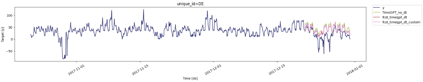
all_fcst = (
    fcst_timegpt_no_dt
    .merge(fcst_timegpt_dt, on=['unique_id', 'ds'])
    .merge(fcst_timegpt_dt_custom, on=['unique_id', 'ds'])
)
all_fcst.head()

nixtla_client.plot(df_sub, all_fcst)

Visually looking at the results shows that the forecast with the datetime features is closer to the actuals as compared to the forecast without the datetime features.

​

Metric Comparison

Next, let’s compare the forecast with the actual data quantitatively. We will use two common metrics - MAE and RMSE for this purpose.

all_fcst_with_actuals = (
    df_test[["unique_id", "ds", "y"]]
    .merge(all_fcst, on=['unique_id', 'ds'])
)
all_fcst_with_actuals.head()

metrics = [mae, rmse]

evaluation = evaluate(
    all_fcst_with_actuals,
    metrics=metrics,
)
evaluation

As we can see, the addition of the datetime features improved the forecasting metrics compared to the baseline model created without these features.

​

Conclusion

As demonstrated in this tutorial

1. Providing datetime features to the model during forecasting can improve the metrics substantially.
2. However, users must be careful of the cardinality of the features after datetime features have been added. If the feature cardinality is too large for the dataset, it may lead to overfitting.
3. In case of high cardinality, users may consider a custom encoding approach as demonstrated.