What Are Categorical Variables?
Categorical variables are external factors that take on a limited range of discrete values, grouping observations by categories. For example, “Sporting” or “Cultural” events in a dataset describing product demand. By capturing unique external conditions, categorical variables enhance the predictive power of your model and can reduce forecasting error. They are easy to incorporate by merging each time series data point with its corresponding categorical data. This tutorial demonstrates how to incorporate categorical (discrete) variables into TimeGPT forecasts.How to Use Categorical Variables in TimeGPT
Step 1: Import Packages and Initialize the Nixtla Client
Make sure you have the necessary libraries installed: pandas, nixtla, and datasetsforecast.Step 2: Load M5 Data
We use the M5 dataset — a collection of daily product sales demands across 10 US stores — to showcase how categorical variables can improve forecasts. Start by loading the M5 dataset and converting the date columns to datetime objects.| unique_id | ds | y |
|---|---|---|
| FOODS_1_001_CA_1 | 2011-01-29 | 3.0 |
| FOODS_1_001_CA_1 | 2011-01-30 | 0.0 |
| FOODS_1_001_CA_1 | 2011-01-31 | 0.0 |
| FOODS_1_001_CA_1 | 2011-02-01 | 1.0 |
| FOODS_1_001_CA_1 | 2011-02-02 | 4.0 |
| FOODS_1_001_CA_1 | 2011-02-03 | 2.0 |
| FOODS_1_001_CA_1 | 2011-02-04 | 0.0 |
| FOODS_1_001_CA_1 | 2011-02-05 | 2.0 |
| FOODS_1_001_CA_1 | 2011-02-06 | 0.0 |
| FOODS_1_001_CA_1 | 2011-02-07 | 0.0 |
| unique_id | ds | event_type_1 |
|---|---|---|
| FOODS_1_001_CA_1 | 2011-01-29 | nan |
| FOODS_1_001_CA_1 | 2011-01-30 | nan |
| FOODS_1_001_CA_1 | 2011-01-31 | nan |
| FOODS_1_001_CA_1 | 2011-02-01 | nan |
| FOODS_1_001_CA_1 | 2011-02-02 | nan |
| FOODS_1_001_CA_1 | 2011-02-03 | nan |
| FOODS_1_001_CA_1 | 2011-02-04 | nan |
| FOODS_1_001_CA_1 | 2011-02-05 | nan |
| FOODS_1_001_CA_1 | 2011-02-06 | Sporting |
| FOODS_1_001_CA_1 | 2011-02-07 | nan |
event_type_1.
Step 3: Prepare Data for Forecasting
We’ll select a specific product to demonstrate how to incorporate categorical features into TimeGPT forecasts.Select a High-Selling Product and Merge Data
Start by selecting a high-selling product and merging the data.| unique_id | ds | y | event_type_1 |
|---|---|---|---|
| FOODS_3_090_CA_3 | 2011-01-29 | 108.0 | nan |
| FOODS_3_090_CA_3 | 2011-01-30 | 132.0 | nan |
| FOODS_3_090_CA_3 | 2011-01-31 | 102.0 | nan |
| FOODS_3_090_CA_3 | 2011-02-01 | 120.0 | nan |
| FOODS_3_090_CA_3 | 2011-02-02 | 106.0 | nan |
| FOODS_3_090_CA_3 | 2011-02-03 | 123.0 | nan |
| FOODS_3_090_CA_3 | 2011-02-04 | 279.0 | nan |
| FOODS_3_090_CA_3 | 2011-02-05 | 175.0 | nan |
| FOODS_3_090_CA_3 | 2011-02-06 | 186.0 | Sporting |
| FOODS_3_090_CA_3 | 2011-02-07 | 120.0 | nan |
Prepare Future External Variables
Select future external variables for Feb 1-7, 2016.| unique_id | ds | y | event_type_1 |
|---|---|---|---|
| FOODS_3_090_CA_3 | 2016-01-22 | 94.0 | nan |
| FOODS_3_090_CA_3 | 2016-01-23 | 144.0 | nan |
| FOODS_3_090_CA_3 | 2016-01-24 | 146.0 | nan |
| FOODS_3_090_CA_3 | 2016-01-25 | 87.0 | nan |
| FOODS_3_090_CA_3 | 2016-01-26 | 73.0 | nan |
| FOODS_3_090_CA_3 | 2016-01-27 | 62.0 | nan |
| FOODS_3_090_CA_3 | 2016-01-28 | 64.0 | nan |
| FOODS_3_090_CA_3 | 2016-01-29 | 102.0 | nan |
| FOODS_3_090_CA_3 | 2016-01-30 | 113.0 | nan |
| FOODS_3_090_CA_3 | 2016-01-31 | 98.0 | nan |
Step 4: Forecast Product Demand
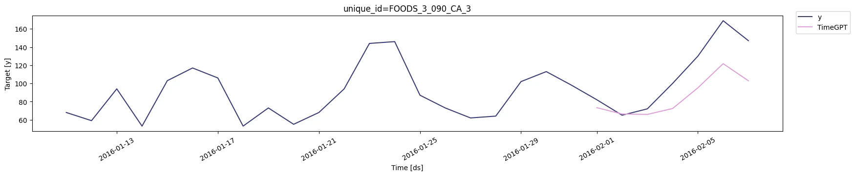
To evaluate the impact of categorical variables, we’ll forecast product demand with and without them.Forecast Without Categorical Variables
| unique_id | ds | TimeGPT | TimeGPT-hi-80 | TimeGPT-hi-90 | TimeGPT-lo-80 | TimeGPT-lo-90 |
|---|---|---|---|---|---|---|
| FOODS_3_090_CA_3 | 2016-02-01 | 73.304090 | 95.887380 | 98.250880 | 50.720802 | 48.357307 |
| FOODS_3_090_CA_3 | 2016-02-02 | 66.335520 | 75.429660 | 76.663704 | 57.241375 | 56.007330 |
| FOODS_3_090_CA_3 | 2016-02-03 | 65.881630 | 86.636480 | 87.502810 | 45.126778 | 44.260456 |
| FOODS_3_090_CA_3 | 2016-02-04 | 72.371864 | 92.362690 | 96.378610 | 52.381035 | 48.365116 |
| FOODS_3_090_CA_3 | 2016-02-05 | 95.141045 | 111.439224 | 114.115490 | 78.842865 | 76.166595 |
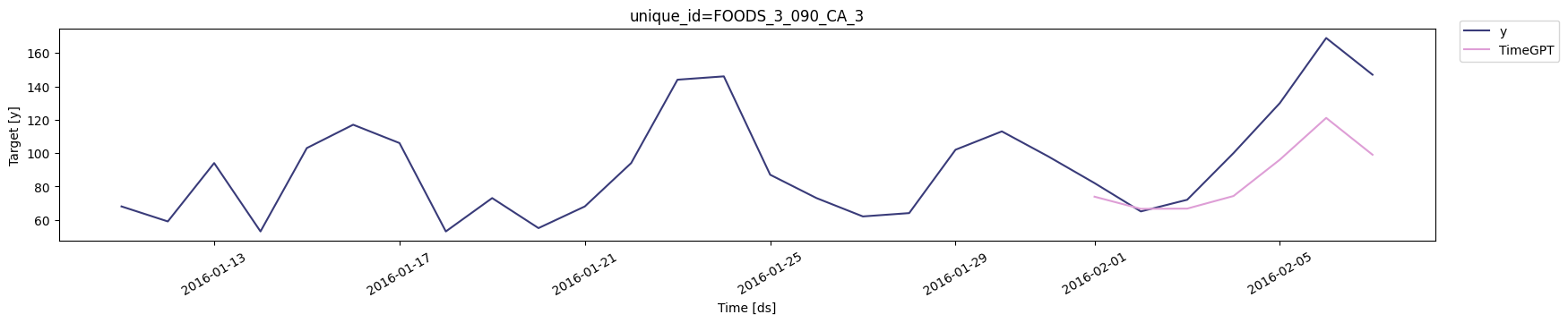
Forecast With Categorical Variables
To forecast with categorical variables, simply provide the list of column names containing categorical features in thecategorical_exog_list argument.
| unique_id | ds | TimeGPT | TimeGPT-hi-80 | TimeGPT-hi-90 | TimeGPT-lo-80 | TimeGPT-lo-90 |
|---|---|---|---|---|---|---|
| FOODS_3_090_CA_3 | 2016-02-01 | 73.839455 | 100.905910 | 104.44151 | 46.773006 | 43.237396 |
| FOODS_3_090_CA_3 | 2016-02-02 | 66.548750 | 75.294970 | 76.62822 | 57.802540 | 56.469284 |
| FOODS_3_090_CA_3 | 2016-02-03 | 66.694435 | 87.777954 | 88.63922 | 45.610912 | 44.749650 |
| FOODS_3_090_CA_3 | 2016-02-04 | 74.249530 | 94.813286 | 98.88473 | 53.685770 | 49.614326 |
| FOODS_3_090_CA_3 | 2016-02-05 | 96.052414 | 112.402090 | 115.22341 | 79.702736 | 76.881420 |
5. Evaluate Forecast Accuracy
Finally, we calculate the Symmetric Mean Absolute Percentage Error (sMAPE) for the forecasts with and without categorical variables.| unique_id | TimeGPT-without-cat-vars | TimeGPT-with-cat-vars |
|---|---|---|
| FOODS_3_090_CA_3 | 0.109241 | 0.108666 |
Conclusion
Categorical variables are powerful additions to TimeGPT forecasts, helping capture valuable external factors. By simply passing them to thecategorical_exog_list parameter, you can significantly enhance predictive performance.
Continue exploring more advanced techniques or different datasets to further improve your TimeGPT forecasting models.