What is Temporal Hierarchical Forecasting?
Temporal hierarchical forecasting is a technique that improves prediction accuracy by leveraging the structure of time series data across multiple temporal resolutions such as hourly, daily, weekly, and monthly. Rather than modeling just one time scale, it generates forecasts at each level of the temporal hierarchy and then reconciles them to ensure consistency (e.g., the sum of hourly forecasts aligns with the daily total). This approach captures both high-frequency variations and long-term trends, allowing for coherent forecasts across time scales. It is particularly effective in domains like energy demand, retail sales, and transportation planning, where decisions depend on both granular and aggregated time-based insights.Tutorial
Step 1: Import and Initialize
Let’s import the NixtlaClient and Initialize it with an API key.Step 2: Load and Prepare Data
First, let’s read and process the dataset.
Step 3: Temporal Hierarchical Forecasting
Temporal Aggregation
We are interested in generating forecasts for the hourly and 2-hourly windows. We can generate these forecasts using TimeGPT. After generating these forecasts, we make use of hierarchical forecasting techniques to improve the accuracy of each forecast. We first define the temporal aggregation spec. The spec is a dictionary in which the keys are the name of the aggregation and the value is the amount of bottom-level timesteps that should be aggregated in that aggregation. In this example, we choose a temporal aggregation of a 2-hour period and a 1-hour period (the bottom level).Y_train contains our training data, for both 1-hour and 2-hour periods.
For example, if we look at the first two timestamps of the training data,
we have a 2-hour period ending at 2017-10-22 01:00, and two 1-hour periods,
the first ending at 2017-10-22 00:00, and the second at 2017-10-22 01:00,
the latter corresponding to when the first 2-hour period ends.
Also, the ground truth value y of the first 2-hour period is 38.13, which
is equal to the sum of the first two 1-hour periods (19.10 + 19.03). This
showcases how the higher frequency 1-hour-period has been aggregated into
the 2-hour-period frequency.
The aggregation matrices
S_train and S_test detail how the lowest temporal
granularity (hour) can be aggregated into the 2-hour periods. For example,
the first 2-hour period, named 2-hour-period-1, can be constructed by
summing the first two hour-periods, 1-hour-period-1 and 1-hour-period-2,
which we also verified above in our inspection of Y_train.
Computing Base Forecasts with TimeGPT
Now, we need to compute base forecasts for each temporal aggregation. The following cell computes the base forecasts for each temporal aggregation inY_train using TimeGPT.
Note that both frequency and horizon are different for each temporal
aggregation. In this example, the lowest level has a hourly frequency, and a
horizon of 48. The 2-hourly-period aggregation thus has a 2-hourly
frequency with a horizon of 24.
Y_hat contains all the forecasts but they are not coherent
with each other. For example, consider the forecasts for the first time
period of both frequencies.
The ground truth value
y for the first 2-hour period is 10.45, and the sum
of the ground truth values for the first two 1-hour periods is (9.73 + 0.72)
= 10.45. Hence, these values are coherent with each other.
However, the forecast for the first 2-hour period is 16.95, but the sum of
the forecasts for the first two 1-hour periods is -3.69. Hence, these
forecasts are clearly not coherent with each other.
We will use reconciliation techniques to make these forecasts better
coherent with each other and improve their accuracy.
Forecast Reconciliation
We can use theHierarchicalReconciliation class to reconcile the forecasts.
In this example we use MinTrace. Note that we have to set temporal=True
in the reconcile function.
The
S parameter was renamed to S_df in hierarchicalforecast. Make sure
you are using S_df when calling reconcile.Step 4. Evaluation
TheHierarchicalForecast package includes the evaluate function to
evaluate the different hierarchies.
We evaluate the temporally aggregated forecasts across all temporal aggregations.
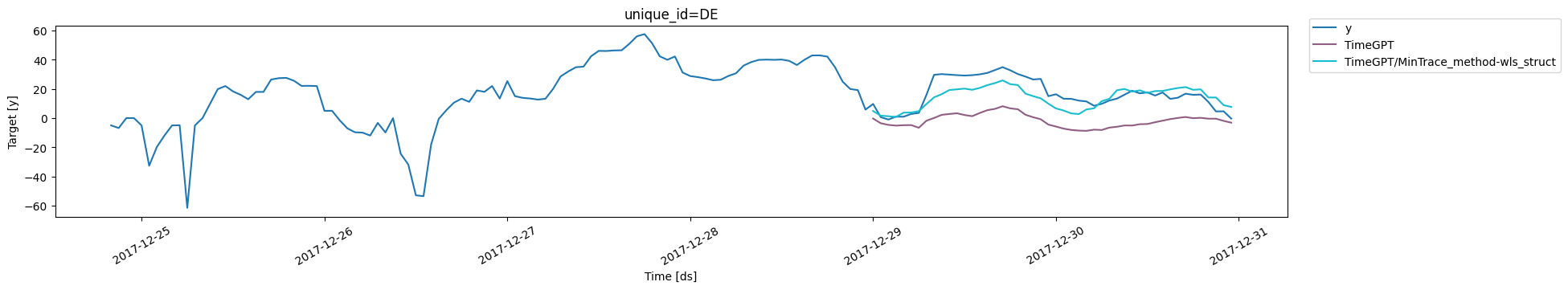
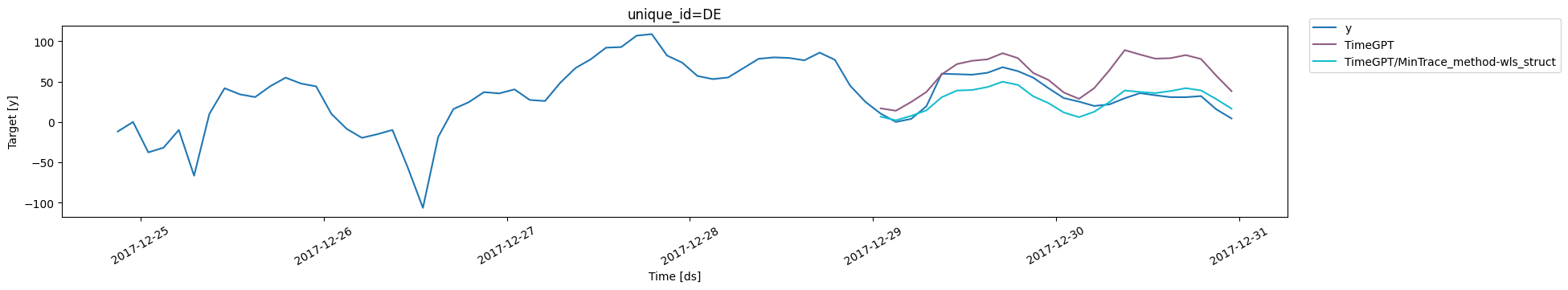
As we can see, we improved performance of TimeGPT’s predictions both for the
2-hour period and for the 1-hour period, as both levels see a significant
reduction in MAE.
Visually, we can also verify the forecast is better after using reconciliation
techniques.
For the 1-hour-period forecasts:
Conclusion
In this tutorial we have shown:- How to create forecasts for multiple frequencies for the same dataset with TimeGPT
- How to improve the accuracy of these forecasts using temporal reconciliation techniques