Introduction
Energy demand forecasting is critical for grid operations, resource allocation, and infrastructure planning. Despite advances in methods, predicting consumption remains challenging due to weather, economic activity, and consumer behavior. This tutorial demonstrates how TimeGPT simplifies in-zone electricity forecasting while delivering superior accuracy and speed. We will use the PJM Hourly Energy Consumption dataset covering five regions from October 2023 to September 2024.What You’ll Learn
- How to load and prepare energy consumption data
- How to generate 4-day ahead forecasts with TimeGPT
- How to evaluate forecast accuracy using MAE and sMAPE
- How TimeGPT compares to deep learning models like N-HiTS
How to Use TimeGPT to Forecast Energy Demand
Step 1: Initial Setup
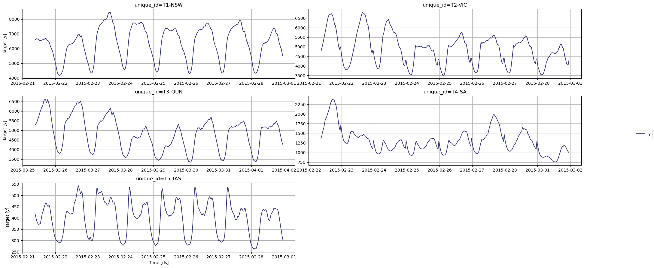
Install and import required packages, then create a NixtlaClient instance to interact with TimeGPT.Step 2: Load Energy Consumption Data
Load the energy consumption dataset and convert datetime strings to timestamps.| unique_id | ds | y | |
|---|---|---|---|
| 0 | AP-AP | 2023-10-01 04:00:00+00:00 | 4042.513 |
| 1 | AP-AP | 2023-10-01 05:00:00+00:00 | 3850.067 |
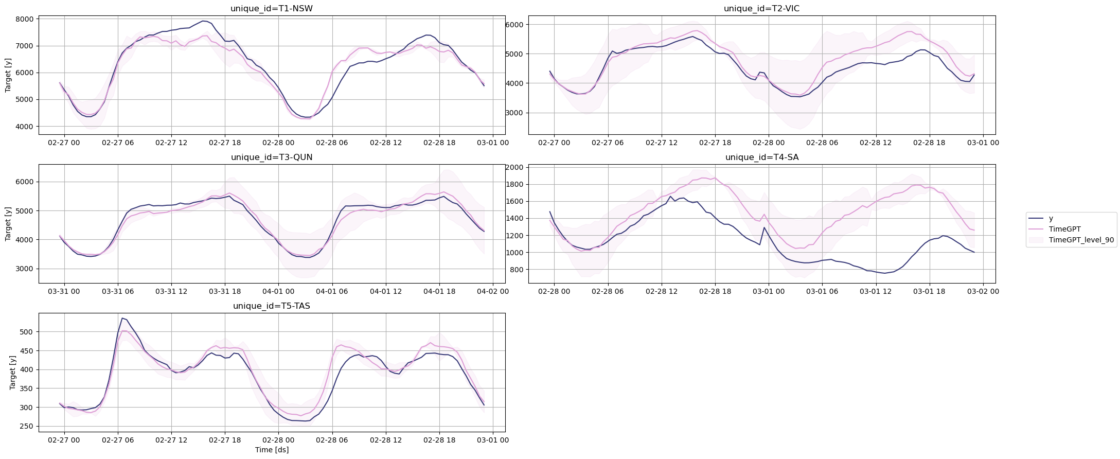
Step 3: Generate Energy Demand Forecasts with TimeGPT
We’ll split our dataset into:- A training/input set for model calibration
- A testing set (last 4 days) to validate performance
Step 4: Evaluate Forecast Accuracy
Compute accuracy metrics (MAE and sMAPE) for TimeGPT.Step 5: Forecast with N-HiTS
For comparison, we train and forecast using the deep-learning model N-HiTS.Step 6: Evaluate N-HiTS
Compute accuracy metrics (MAE and sMAPE) for N-HiTS.Conclusion
TimeGPT demonstrates substantial performance improvements over N-HiTS across key metrics:- Accuracy: 18.6% lower MAE (882.6 vs 1084.7)
- Error Rate: 31.1% lower sMAPE
- Speed: 90% faster predictions (4.3 seconds vs 44 seconds)
Related Tutorials
Ready to explore more forecasting applications? Check out these guides:- Bitcoin Price Prediction with TimeGPT - Financial time series forecasting
- Exogenous Variables Guide - Improve forecasts with external data
- Long Horizon Forecasting - Extended forecast periods