Overview
When monitoring multiple time series simultaneously, such as server metrics (CPU, memory, disk I/O), you need to choose between local and global anomaly detection strategies. This guide demonstrates:- Local (Univariate) Detection: Analyzing each time series independently for isolated metric anomalies
- Global (Multivariate) Detection: Analyzing all time series collectively to detect system-wide failures
detect_anomalies_online with the threshold_method parameter. The main difference is whether anomalies are identified individually per series (local) or collectively across multiple correlated series (global).
For an introduction to real-time anomaly detection, see our Real-Time Anomaly Detection guide. To learn about parameter tuning, check out Controlling the Anomaly Detection Process.
When to Use Each Method
Use Local Detection When:
- Monitoring independent, uncorrelated metrics
- Each metric has distinct baseline behavior
- You need low computational overhead
- False positives in individual series are acceptable
Use Global Detection When:
- Monitoring correlated server or system metrics
- System-wide failures affect multiple metrics simultaneously
- You need to detect coordinated anomalies (e.g., CPU spike + memory spike + network spike)
- Reducing false positives by considering metric relationships
How to Detect Anomalies Across Multiple Time Series
Step 1: Set Up Your Environment
Import dependencies that you will use in the tutorial.Step 2: Load the Dataset
This tutorial uses the SMD (Server Machine Dataset), a benchmark dataset for anomaly detection across multiple time series. SMD monitors abnormal patterns in server machine data. We analyze monitoring data from a single server (machine-1-1) containing 38 time series. Each series represents a different server metric: CPU usage, memory usage, disk I/O, network throughput, and other system performance indicators.Step 3: Local and Global Anomaly Detection Methods
Method Comparison
Step 3.1: Local Method
Local anomaly detection analyzes each time series in isolation, flagging anomalies based on each series’ individual deviation from its expected behavior. This approach is efficient for individual metrics or when correlations between metrics are not relevant. However, it may miss large-scale, system-wide anomalies that are only apparent when multiple series deviate simultaneously. Example usage:
Local Anomaly Detection Results
Step 3.2: Global Method
Global anomaly detection considers all time series collectively, flagging a time step as anomalous if the aggregate deviation across all series at that time exceeds a threshold. This approach captures systemic or correlated anomalies that might be missed when analyzing each series in isolation. However, it comes with slightly higher complexity and computational overhead, and may require careful threshold tuning. Example usage: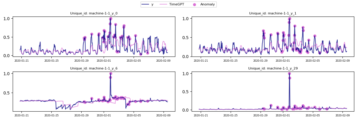
Global Anomaly Detection Results
Real-World Use Cases
Local Detection Examples:
- Independent application metrics: Response time, error rates, request counts for different microservices
- IoT sensor networks: Temperature sensors at different locations with no correlation
- Business metrics: Sales figures across different product categories
Global Detection Examples:
- Server monitoring: CPU, memory, disk I/O, and network metrics from the same server
- Distributed system health: Correlated metrics across multiple nodes indicating cluster-wide issues
- Manufacturing equipment: Multiple sensor readings from a single machine indicating equipment failure
Summary
- Local: Best for detecting anomalies in a single metric or uncorrelated metrics. Low computational overhead, but may overlook cross-series patterns.
- Global: Considers correlations across metrics, capturing system-wide issues. More complex and computationally intensive than local methods.
Frequently Asked Questions
What’s the difference between univariate and multivariate anomaly detection? Univariate (local) detection analyzes each time series independently using thethreshold_method='univariate' parameter, while multivariate (global) detection analyzes all series together using threshold_method='multivariate', considering correlations between metrics.
When should I use global detection instead of local?
Use global detection when your time series are correlated and system-wide failures affect multiple metrics simultaneously, such as monitoring CPU, memory, and network metrics from the same server.
Does global detection increase computational cost?
Yes, global detection requires analyzing relationships across all time series, making it more computationally intensive. However, it can reduce overall false positives by considering metric correlations.
Can I run both local and global detection?
Yes, you can run both methods and compare results. Local detection may catch metric-specific anomalies while global detection identifies system-wide issues.