Forecasting 145,000 Time Series in 7 Minutes with TimeGPT

What if you could forecast every Wikipedia article's daily traffic — 145,000 time series — without writing a single feature engineering pipeline? No seasonality decomposition, no hyperparameter search, no training loop. Just an API call.

That's the promise of TimeGPT. In this post, we put it to the test on the Kaggle Web Traffic Time Series Forecasting competition, benchmarking it against a strong statistical baseline. The result: all 145,063 series forecasted in 6.6 minutes, beating the baseline by more than 8 SMAPE points — with a single API call per language batch.

The Dataset

The competition provides daily page view counts for 145,063 Wikipedia articles spanning July 2015 to September 2017 (~800 days). The series cover seven languages (English, Japanese, German, French, Chinese, Russian, Spanish) and multiple access types (desktop, mobile, all-access) and agent types (human, bot, spider).

This diversity is what makes the dataset hard. A single model has to handle everything from the English Wikipedia homepage (millions of daily views, strong weekly seasonality) to an obscure article in Russian (sparse, near-zero for months, then a sudden spike).

The competition metric is SMAPE (Symmetric Mean Absolute Percentage Error), which penalizes both over- and under-forecasting symmetrically:

$$\text{SMAPE} = \frac{100\%}{n} \sum_{t=1}^{n} \frac{|y_t - \hat{y}_t|}{(|y_t| + |\hat{y}_t|) / 2}$$

Experimental Setup

Rather than forecasting the held-out competition test set, we do a proper train/validation split on the training data itself:

• Training window: first 743 days (2015-07-01 → 2017-07-10)
• Validation window: last 60 days (2017-07-11 → 2017-09-09)
• All 145,063 series — no sampling

Both methods see exactly the same training data and are evaluated on the same 60-day validation window.

def train_val_split(df_wide: pd.DataFrame, h: int):
    date_cols  = [c for c in df_wide.columns if c != "Page"]
    train_cols = date_cols[:-h]
    val_cols   = date_cols[-h:]
    df_train   = df_wide[["Page"] + train_cols].copy()
    df_val     = df_wide[["Page"] + val_cols].copy()
    return df_train, df_val

df_train, df_val = train_val_split(df_wide, h=60)

The Baseline: Fibonacci Median

Our baseline is a highly voted Kaggle kernel by safavieh, which achieved a public leaderboard score of ~44.9 SMAPE — a top result using zero machine learning.

The idea is elegant: instead of fitting a model, compute the median of several trailing windows whose sizes follow Fibonacci-like spacing — [6, 12, 18, 30, 48, 78, 126, 203, 329] days. Take the median of those medians. Use that single number as a flat forecast for all future days.

GOLDEN_WINDOWS = [6, 12, 18, 30, 48, 78, 126, 203, 329]

def golden_median(values: np.ndarray) -> float:
    # Skip leading zeros so sparse series don't anchor too low
    start = np.nonzero(values)[0]
    if len(start) == 0:
        return 0.0
    active = values[start[0]:]
    n = len(active)
    if n < GOLDEN_WINDOWS[0]:
        return float(np.median(active))
    medians = [np.median(active[-w:]) for w in GOLDEN_WINDOWS if w <= n]
    return float(np.median(medians))

Applied to all 145,063 series, this runs in 8.4 seconds and achieves a mean SMAPE of 43.03% on our validation set. Remarkably fast and strong for a method with no model fitting whatsoever.

TimeGPT: Zero-Shot Forecasting

TimeGPT is a foundation model for time series, pretrained on a large dataset of real-world time series spanning many domains and frequencies. The key property for this task: it requires no fine-tuning and no feature engineering. You hand it your training data, specify the horizon, and it forecasts.

To keep each API call manageable, we batch by language — 7 batches ranging from ~14K to ~24K series each:

from nixtla import NixtlaClient

client = NixtlaClient(api_key="your_api_key")

LANGUAGES = ["en", "ja", "de", "fr", "zh", "ru", "es"]

for lang in LANGUAGES:
    mask    = df_train["Page"].str.contains(f"_{lang}.wikipedia.org_", regex=False)
    df_lang = df_train[mask]

    # Reshape from competition's wide format to long format
    df_long = wide_to_long(df_lang)  # columns: unique_id, ds, y

    fcst = client.forecast(
        df=df_long,
        h=60,
        freq="D",
        time_col="ds",
        target_col="y",
        id_col="unique_id",
        model="timegpt-2.1",
    )

No seasonality flags, no lag selection, no hyperparameters. Each language batch is a single API call.

Results

TimeGPT reduces mean SMAPE from 43.03% to 34.92% — an 18.8% relative improvement over the Fibonacci baseline — across all 145,063 series in under 7 minutes.

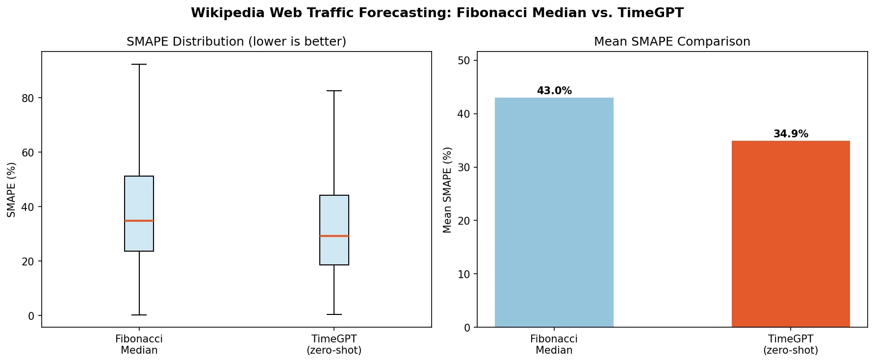
The box plots tell the fuller story: TimeGPT doesn't just improve on average, it achieves a substantially lower median (29.28% vs. 34.80%), meaning it handles the majority of series much better. Both methods encounter the same hard cases — extremely sparse or highly volatile series — but TimeGPT's distribution is tighter and shifted meaningfully lower.

Speed in Context

The timeline for this entire experiment:

For comparison, a classical ML approach on this dataset — building lag features, rolling statistics, Fourier transforms, and holiday calendars per language, then training and cross-validating a gradient boosting model — typically takes days of development followed by hours of compute.

With TimeGPT, the path from raw data to a validated, competitive forecast is measured in minutes, not days.

Reproducing This

# 1. Install dependencies
pip install nixtla pandas matplotlib python-dotenv kaggle

# 2. Download data (requires Kaggle credentials at ~/.kaggle/kaggle.json)
kaggle competitions download -c web-traffic-time-series-forecasting -p data/wiki
unzip data/wiki/web-traffic-time-series-forecasting.zip -d data/wiki
unzip data/wiki/train_2.csv.zip -d data/wiki

# 3. Run the full benchmark
NIXTLA_API_KEY=your_key python wiki_traffic_forecast.py --model timegpt-2.1

The complete script is available as a GitHub Gist.

Takeaway

TimeGPT is not just fast at inference — it's fast from idea to result. The entire experiment in this post, from raw CSV to a validated comparison against a top Kaggle statistical baseline, takes under 7 minutes of wall-clock time — no training, no feature engineering, no hyperparameter search.

For teams that need a competitive starting point quickly — before investing in custom feature pipelines — TimeGPT offers a compelling first step. An 18.8% accuracy improvement over a well-tuned statistical baseline comes for free, with no domain expertise required.

Get started with TimeGPT →