> ## Documentation Index
> Fetch the complete documentation index at: https://nixtla.io/docs/llms.txt
> Use this file to discover all available pages before exploring further.
# Forecasting Intermittent Demand
> Master intermittent demand forecasting with TimeGPT for inventory optimization. Achieve 14% better accuracy than specialized models using the M5 dataset with exogenous variables and log transforms.
## Introduction
Intermittent demand occurs when products or services have irregular purchase patterns with frequent zero-value periods. This is common in retail, spare parts inventory, and specialty products where demand is irregular rather than continuous.
Forecasting these patterns accurately is essential for optimizing stock levels, reducing costs, and preventing stockouts. [TimeGPT](/introduction/about_timegpt) excels at intermittent demand forecasting by capturing complex patterns that traditional statistical methods miss.
This tutorial demonstrates TimeGPT's capabilities using the M5 dataset of food sales, including [exogenous variables](/forecasting/exogenous-variables/numeric_features) like pricing and promotional events that influence purchasing behavior.
### What You'll Learn
* How to prepare and analyze intermittent demand data
* How to leverage exogenous variables for better predictions
* How to use log transforms to ensure realistic forecasts
* How TimeGPT compares to specialized intermittent demand models
The methods shown here apply broadly to inventory management and retail forecasting challenges. For getting started with TimeGPT, see our [quickstart guide](/forecasting/timegpt_quickstart).
## How to Use TimeGPT to Forecast Intermittent Demand
[](https://colab.research.google.com/github/Nixtla/nixtla/blob/main/nbs/docs/use-cases/4_intermittent_demand.ipynb)
### Step 1: Environment Setup
Start by importing the required packages for this tutorial and create an instance of `NixtlaClient`.
```python theme={null}
import pandas as pd
import numpy as np
from nixtla import NixtlaClient
from utilsforecast.losses import mae
from utilsforecast.evaluation import evaluate
nixtla_client = NixtlaClient(api_key='my_api_key_provided_by_nixtla')
```
### Step 2: Load and Visualize the Dataset
Load the dataset from the M5 dataset and convert the `ds` column to a datetime object:
```python theme={null}
df = pd.read_csv("https://raw.githubusercontent.com/Nixtla/transfer-learning-time-series/main/datasets/m5_sales_exog_small.csv")
df['ds'] = pd.to_datetime(df['ds'])
df.head()
```
| unique\_id | ds | y | sell\_price | event\_type\_Cultural | event\_type\_National | event\_type\_Religious | event\_type\_Sporting |
| ------------- | ---------- | - | ----------- | --------------------- | --------------------- | ---------------------- | --------------------- |
| FOODS\_1\_001 | 2011-01-29 | 3 | 2.0 | 0 | 0 | 0 | 0 |
| FOODS\_1\_001 | 2011-01-30 | 0 | 2.0 | 0 | 0 | 0 | 0 |
| FOODS\_1\_001 | 2011-01-31 | 0 | 2.0 | 0 | 0 | 0 | 0 |
| FOODS\_1\_001 | 2011-02-01 | 1 | 2.0 | 0 | 0 | 0 | 0 |
| FOODS\_1\_001 | 2011-02-02 | 4 | 2.0 | 0 | 0 | 0 | 0 |
Visualize the dataset using the `plot` method:
```python theme={null}
nixtla_client.plot(
df,
max_insample_length=365,
)
```
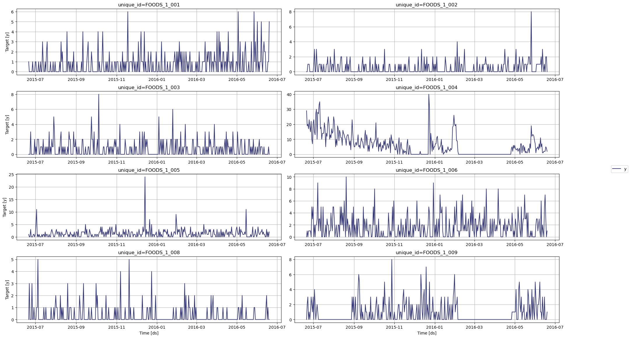
In the figure above, we can see the intermittent nature of this dataset, with many periods with zero demand.
Now, let's use TimeGPT to forecast the demand of each product.
### Step 3: Transform the Data
To avoid getting negative predictions coming from the model, we use a log transformation on the data. That way, the model will be forced to predict only positive values.
Note that due to the presence of zeros in our dataset, we add one to all points before taking the log.
```python theme={null}
df_transformed = df.copy()
df_transformed['y'] = np.log(df_transformed['y'] + 1)
```
Now, let's keep the last 28 time steps for the test set and use the rest as input to the model.
```python theme={null}
test_df = df_transformed.groupby('unique_id').tail(28)
input_df = df_transformed.drop(test_df.index).reset_index(drop=True)
```
### Step 4: Forecast with TimeGPT
Forecast with TimeGPT using the `forecast` method:
```python theme={null}
fcst_df = nixtla_client.forecast(
df=input_df,
h=28,
level=[80],
finetune_steps=10, # Learn more about fine-tuning: /forecasting/fine-tuning/steps
finetune_loss='mae',
model='timegpt-1-long-horizon', # For long-horizon forecasting: /forecasting/model-version/longhorizon_model
time_col='ds',
target_col='y',
id_col='unique_id'
)
```
```bash theme={null}
INFO:nixtla.nixtla_client:Validating inputs...
INFO:nixtla.nixtla_client:Preprocessing dataframes...
INFO:nixtla.nixtla_client:Inferred freq: D
INFO:nixtla.nixtla_client:Calling Forecast Endpoint...
```
Great! We now have predictions. However, those predictions are transformed, so we need to inverse the transformation to get back to the original scale. Therefore, we take the exponential and subtract one from each data point.
```python theme={null}
cols = [col for col in fcst_df.columns if col not in ['ds', 'unique_id']]
fcst_df[cols] = np.exp(fcst_df[cols]) - 1
fcst_df.head()
```
| | unique\_id | ds | TimeGPT | TimeGPT-lo-80 | TimeGPT-hi-80 |
| - | ------------- | ---------- | -------- | ------------- | ------------- |
| 0 | FOODS\_1\_001 | 2016-05-23 | 0.286841 | -0.267101 | 1.259465 |
| 1 | FOODS\_1\_001 | 2016-05-24 | 0.320482 | -0.241236 | 1.298046 |
| 2 | FOODS\_1\_001 | 2016-05-25 | 0.287392 | -0.362250 | 1.598791 |
| 3 | FOODS\_1\_001 | 2016-05-26 | 0.295326 | -0.145489 | 0.963542 |
| 4 | FOODS\_1\_001 | 2016-05-27 | 0.315868 | -0.166516 | 1.077437 |
### Step 5: Evaluate the Forecasts
Before measuring the performance metric, let's plot the predictions against the actual values.
```python theme={null}
nixtla_client.plot(
test_df,
fcst_df,
models=['TimeGPT'],
level=[80],
time_col='ds',
target_col='y'
)
```
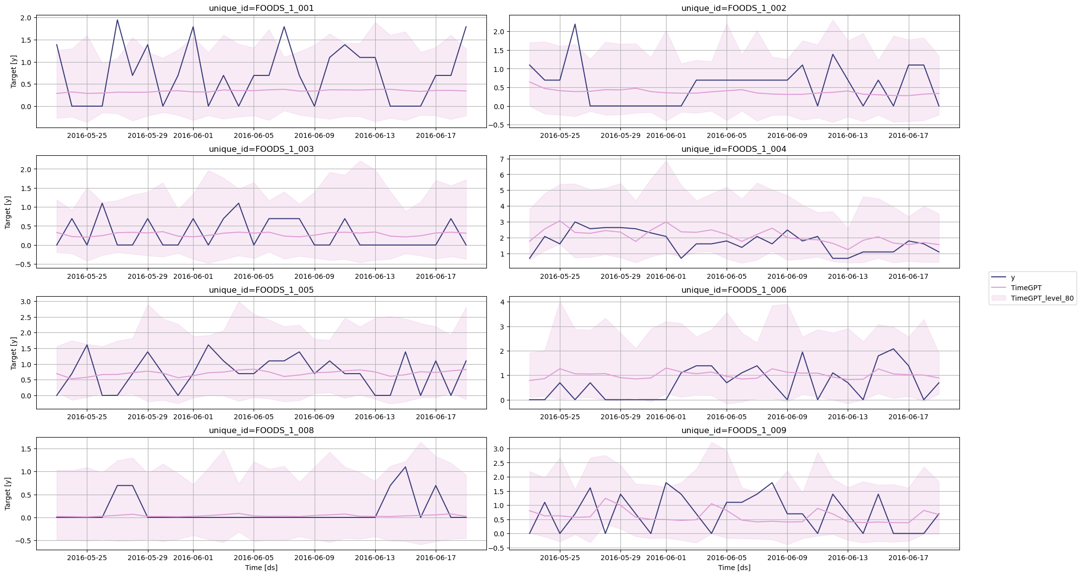
Finally, we can measure the mean absolute error (MAE) of the model. Learn more about [evaluation metrics](/forecasting/evaluation/evaluation_metrics) in our documentation.
```python theme={null}
# Compute MAE
test_df = pd.merge(test_df, fcst_df, how='left', on=['unique_id', 'ds'])
evaluation = evaluate(
test_df,
metrics=[mae],
models=['TimeGPT'],
target_col='y',
id_col='unique_id'
)
average_metrics = evaluation.groupby('metric')['TimeGPT'].mean()
average_metrics
```
```bash theme={null}
metric
mae 0.492559
```
### Step 6: Compare with Statistical Models
The library `statsforecast` by Nixtla provides a suite of statistical models specifically built for intermittent forecasting, such as Croston, IMAPA and TSB. Let's use these models and see how they perform against TimeGPT.
```python theme={null}
from statsforecast import StatsForecast
from statsforecast.models import CrostonClassic, CrostonOptimized, IMAPA, TSB
sf = StatsForecast(
models=[CrostonClassic(), CrostonOptimized(), IMAPA(), TSB(0.1, 0.1)],
freq='D',
n_jobs=-1
)
```
Then, we can fit the models on our data.
```python theme={null}
sf.fit(df=input_df)
sf_preds = sf.predict(h=28)
```
Again, we need to inverse the transformation. Remember that the training data was previously transformed using the log function.
```python theme={null}
cols = [col for col in sf_preds.columns if col not in ['ds', 'unique_id']]
sf_preds[cols] = np.exp(sf_preds[cols]) - 1
sf_preds.head()
```
| | unique\_id | ds | CrostonClassic | CrostonOptimized | IMAPA | TSB |
| - | ------------- | ---------- | -------------- | ---------------- | -------- | -------- |
| 0 | FOODS\_1\_001 | 2016-05-23 | 0.599093 | 0.599093 | 0.445779 | 0.396258 |
| 1 | FOODS\_1\_001 | 2016-05-24 | 0.599093 | 0.599093 | 0.445779 | 0.396258 |
| 2 | FOODS\_1\_001 | 2016-05-25 | 0.599093 | 0.599093 | 0.445779 | 0.396258 |
| 3 | FOODS\_1\_001 | 2016-05-26 | 0.599093 | 0.599093 | 0.445779 | 0.396258 |
| 4 | FOODS\_1\_001 | 2016-05-27 | 0.599093 | 0.599093 | 0.445779 | 0.396258 |
Now, let's combine the predictions from all methods and see which performs best.
```python theme={null}
test_df = pd.merge(test_df, sf_preds, 'left', ['unique_id', 'ds'])
test_df.head()
```
| | unique\_id | ds | y | sell\_price | event\_type\_Cultural | event\_type\_National | event\_type\_Religious | event\_type\_Sporting | TimeGPT | TimeGPT-lo-80 | TimeGPT-hi-80 | CrostonClassic | CrostonOptimized | IMAPA | TSB |
| - | ------------- | ---------- | -------- | ----------- | --------------------- | --------------------- | ---------------------- | --------------------- | -------- | ------------- | ------------- | -------------- | ---------------- | -------- | -------- |
| 0 | FOODS\_1\_001 | 2016-05-23 | 1.386294 | 2.24 | 0 | 0 | 0 | 0 | 0.286841 | -0.267101 | 1.259465 | 0.599093 | 0.599093 | 0.445779 | 0.396258 |
| 1 | FOODS\_1\_001 | 2016-05-24 | 0.000000 | 2.24 | 0 | 0 | 0 | 0 | 0.320482 | -0.241236 | 1.298046 | 0.599093 | 0.599093 | 0.445779 | 0.396258 |
| 2 | FOODS\_1\_001 | 2016-05-25 | 0.000000 | 2.24 | 0 | 0 | 0 | 0 | 0.287392 | -0.362250 | 1.598791 | 0.599093 | 0.599093 | 0.445779 | 0.396258 |
| 3 | FOODS\_1\_001 | 2016-05-26 | 0.000000 | 2.24 | 0 | 0 | 0 | 0 | 0.295326 | -0.145489 | 0.963542 | 0.599093 | 0.599093 | 0.445779 | 0.396258 |
| 4 | FOODS\_1\_001 | 2016-05-27 | 1.945910 | 2.24 | 0 | 0 | 0 | 0 | 0.315868 | -0.166516 | 1.077437 | 0.599093 | 0.599093 | 0.445779 | 0.396258 |
```python theme={null}
statistical_models = ["CrostonClassic", "CrostonOptimized", "IMAPA", "TSB"]
evaluation = evaluate(
test_df,
metrics=[mae],
models=["TimeGPT"] + statistical_models,
target_col="y",
id_col='unique_id'
)
average_metrics = evaluation.groupby('metric')[[
"TimeGPT"] + statistical_models].mean()
average_metrics
```
| metric | TimeGPT | CrostonClassic | CrostonOptimized | IMAPA | TSB |
| ------ | -------- | -------------- | ---------------- | -------- | -------- |
| mae | 0.492559 | 0.564563 | 0.580922 | 0.571943 | 0.567178 |
In the table above, we can see that TimeGPT achieves the lowest MAE, achieving a 12.8% improvement over the best performing statistical model.
These results demonstrate TimeGPT's strong performance without additional features. We can further improve accuracy by incorporating exogenous variables, a capability TimeGPT supports but traditional statistical models do not.
### Step 7: Use Exogenous Variables
To forecast with [exogenous variables](/forecasting/exogenous-variables/numeric_features), we need to specify their future values over the forecast horizon. Therefore, let's simply take the types of events, as those dates are known in advance. You can also explore using [date features](/forecasting/exogenous-variables/date_features) and [holidays](/forecasting/exogenous-variables/holiday_and_special_dates) as exogenous variables.
```python theme={null}
# Include holiday/event data as exogenous features
exog_cols = ['event_type_Cultural', 'event_type_National', 'event_type_Religious', 'event_type_Sporting']
futr_exog_df = test_df[['unique_id', 'ds'] + exog_cols]
futr_exog_df.head()
```
| | unique\_id | ds | event\_type\_Cultural | event\_type\_National | event\_type\_Religious | event\_type\_Sporting |
| - | ------------- | ---------- | --------------------- | --------------------- | ---------------------- | --------------------- |
| 0 | FOODS\_1\_001 | 2016-05-23 | 0 | 0 | 0 | 0 |
| 1 | FOODS\_1\_001 | 2016-05-24 | 0 | 0 | 0 | 0 |
| 2 | FOODS\_1\_001 | 2016-05-25 | 0 | 0 | 0 | 0 |
| 3 | FOODS\_1\_001 | 2016-05-26 | 0 | 0 | 0 | 0 |
| 4 | FOODS\_1\_001 | 2016-05-27 | 0 | 0 | 0 | 0 |
Then, we simply call the `forecast` method and pass the `futr_exog_df` in the `X_df` parameter.
```python theme={null}
fcst_df = nixtla_client.forecast(
df=input_df,
X_df=futr_exog_df,
h=28,
level=[80], # Generate a 80% confidence interval
finetune_steps=10, # Specify the number of steps for fine-tuning
finetune_loss='mae', # Use the MAE as the loss function for fine-tuning
model='timegpt-1-long-horizon', # Use the model for long-horizon forecasting
time_col='ds',
target_col='y',
id_col='unique_id'
)
```
```bash theme={null}
INFO:nixtla.nixtla_client:Validating inputs...
INFO:nixtla.nixtla_client:Preprocessing dataframes...
INFO:nixtla.nixtla_client:Inferred freq: D
INFO:nixtla.nixtla_client:Using the following exogenous variables: event_type_Cultural, event_type_National, event_type_Religious, event_type_Sporting
INFO:nixtla.nixtla_client:Calling Forecast Endpoint...
```
Great! Remember that the predictions are transformed, so we have to inverse the transformation again.
```python theme={null}
fcst_df.rename(columns={'TimeGPT': 'TimeGPT_ex'}, inplace=True)
cols = [col for col in fcst_df.columns if col not in ['ds', 'unique_id']]
fcst_df[cols] = np.exp(fcst_df[cols]) - 1
fcst_df.head()
```
| | unique\_id | ds | TimeGPT\_ex | TimeGPT-lo-80 | TimeGPT-hi-80 |
| - | ------------- | ---------- | ----------- | ------------- | ------------- |
| 0 | FOODS\_1\_001 | 2016-05-23 | 0.281922 | -0.269902 | 1.250828 |
| 1 | FOODS\_1\_001 | 2016-05-24 | 0.313774 | -0.245091 | 1.286372 |
| 2 | FOODS\_1\_001 | 2016-05-25 | 0.285639 | -0.363119 | 1.595252 |
| 3 | FOODS\_1\_001 | 2016-05-26 | 0.295037 | -0.145679 | 0.963104 |
| 4 | FOODS\_1\_001 | 2016-05-27 | 0.315484 | -0.166760 | 1.076830 |
Finally, let's evaluate the performance of TimeGPT with exogenous features.
```python theme={null}
test_df['TimeGPT_ex'] = fcst_df['TimeGPT_ex'].values
test_df.head()
```
| | unique\_id | ds | y | sell\_price | event\_type\_Cultural | event\_type\_National | event\_type\_Religious | event\_type\_Sporting | TimeGPT | TimeGPT-lo-80 | TimeGPT-hi-80 | CrostonClassic | CrostonOptimized | IMAPA | TSB | TimeGPT\_ex |
| - | ------------- | ---------- | -------- | ----------- | --------------------- | --------------------- | ---------------------- | --------------------- | -------- | ------------- | ------------- | -------------- | ---------------- | -------- | -------- | ----------- |
| 0 | FOODS\_1\_001 | 2016-05-23 | 1.386294 | 2.24 | 0 | 0 | 0 | 0 | 0.286841 | -0.267101 | 1.259465 | 0.599093 | 0.599093 | 0.445779 | 0.396258 | 0.281922 |
| 1 | FOODS\_1\_001 | 2016-05-24 | 0.000000 | 2.24 | 0 | 0 | 0 | 0 | 0.320482 | -0.241236 | 1.298046 | 0.599093 | 0.599093 | 0.445779 | 0.396258 | 0.313774 |
| 2 | FOODS\_1\_001 | 2016-05-25 | 0.000000 | 2.24 | 0 | 0 | 0 | 0 | 0.287392 | -0.362250 | 1.598791 | 0.599093 | 0.599093 | 0.445779 | 0.396258 | 0.285639 |
| 3 | FOODS\_1\_001 | 2016-05-26 | 0.000000 | 2.24 | 0 | 0 | 0 | 0 | 0.295326 | -0.145489 | 0.963542 | 0.599093 | 0.599093 | 0.445779 | 0.396258 | 0.295037 |
| 4 | FOODS\_1\_001 | 2016-05-27 | 1.945910 | 2.24 | 0 | 0 | 0 | 0 | 0.315868 | -0.166516 | 1.077437 | 0.599093 | 0.599093 | 0.445779 | 0.396258 | 0.315484 |
```python theme={null}
evaluation = evaluate(
test_df,
metrics=[mae],
models=["TimeGPT"] + statistical_models + ["TimeGPT_ex"],
target_col="y",
id_col='unique_id'
)
average_metrics = (
evaluation.groupby('metric')[["TimeGPT"] + statistical_models + ["TimeGPT_ex"]]
).mean()
average_metrics
```
| metric | TimeGPT | CrostonClassic | CrostonOptimized | IMAPA | TSB | TimeGPT\_ex |
| ------ | -------- | -------------- | ---------------- | -------- | -------- | ----------- |
| mae | 0.492559 | 0.564563 | 0.580922 | 0.571943 | 0.567178 | 0.485352 |
From the table above, we can see that using exogenous features improved the performance of TimeGPT. Now, it represents a 14% improvement over the best statistical model.
## Conclusion
TimeGPT provides a robust solution for forecasting intermittent demand:
* \~14% MAE improvement over specialized models
* Supports exogenous features for enhanced accuracy
By leveraging TimeGPT and combining both internal series patterns and external factors, organizations can achieve more reliable forecasts even for challenging intermittent demands.
### Next Steps
* Explore [other use cases](/use_cases/forecasting_energy_demand) with TimeGPT
* Learn about [probabilistic forecasting](/forecasting/probabilistic/introduction) with prediction intervals
* Scale your forecasts with [distributed computing](/forecasting/forecasting-at-scale/computing_at_scale)
* Fine-tune models with [custom loss functions](/forecasting/fine-tuning/custom_loss)