> ## Documentation Index
> Fetch the complete documentation index at: https://nixtla.io/docs/llms.txt
> Use this file to discover all available pages before exploring further.
# Plan Retail Promotions with Coupled Simulation
> Measure promotion lift, cannibalization, cross-selling, and shared inventory risk across a group of related products.
## Introduction
A store plans a 15% price cut on one product for the next four weeks, and the
category manager needs order quantities for three related products: the promoted
product itself, an alternative product customers might have bought instead, and
a related product often bought alongside it. A promotion rarely affects just one
product. Lowering one price can:
* Increase sales of the promoted product
* Reduce sales of an alternative product through **cannibalization** — shoppers
switch to the cheaper option instead of buying both
* Increase sales of a related product through **cross-selling** — shoppers who
come for the promotion pick up companion items too
This is a follow-on to
[What-If Forecasting: Price Effects in Retail](/docs/use_cases/what_if_forecasting_price_effects_in_retail).
Start there if you first want to see how changing one product's future price
changes its forecast. Continue here when your decision covers several related
products.
This tutorial uses coupled simulation to answer two questions:
1. How could a promotion change demand across a product group?
2. How often could several products need replenishment at the same time?
With coupled simulation, one `sample_id` represents one possible future for the
whole product group. The promoted, alternative, and related products all belong
to the same scenario.
### What You'll Learn
* How to simulate a group of related products together with `multivariate=True`
* How to measure promotion lift, cannibalization, and cross-selling from
simulated paths
* Why simulating products separately understates shared-demand risk
* How to turn a set of simulated futures into ordering decisions
## How to Plan a Promotion with Coupled Simulation
[](https://colab.research.google.com/github/Nixtla/nixtla/blob/main/nbs/docs/use-cases/6_coupled_simulation_retail.ipynb)
### Step 1: Import Packages
Import the required packages and initialize a Nixtla client:
```python theme={null}
import numpy as np
import pandas as pd
from nixtla import NixtlaClient
nixtla_client = NixtlaClient(
# Defaults to os.environ["NIXTLA_API_KEY"]
api_key="my_api_key_provided_by_nixtla"
)
```
### Step 2: Load the Product-Group Data
The example uses three years of daily sales for the three products. Every row
carries all three prices, so when the promoted product's price changes, the
demand simulation for every product can respond. The data is generated rather
than observed — that way the product relationships are known exactly, and the
simulation's answers can be checked against them (see the
[technical notes](#technical-notes) for how, and why, the data was built).
```python theme={null}
rng = np.random.default_rng(11)
n = 1095 # three years of daily history
h = 28 # the promotion window
t = np.arange(n + h)
# Each product runs its own price schedule; the three do not move together.
# Prices carry a lot of day-to-day movement, which is what identifies the price
# effects. Footfall below drifts slowly instead, so the two cannot be confused
# for each other.
promoted_price = (
6.00
+ 0.60 * np.sin(2 * np.pi * t / 97)
+ 0.30 * np.sin(2 * np.pi * t / 29)
+ rng.normal(0, 0.30, n + h)
)
alternative_price = (
9.00
+ 0.85 * np.sin(2 * np.pi * t / 73 + 1.1)
+ 0.40 * np.sin(2 * np.pi * t / 23)
+ rng.normal(0, 0.36, n + h)
)
related_price = (
4.50
+ 0.45 * np.sin(2 * np.pi * t / 113 + 2.3)
+ 0.22 * np.sin(2 * np.pi * t / 31)
+ rng.normal(0, 0.24, n + h)
)
# Store footfall drifts through busy and quiet stretches, lifting every product
# on the same day. It is never given to the model, so it survives as demand that
# moves together across the products.
shock = rng.normal(0, 1, n + h)
footfall = np.zeros(n + h)
for i in range(1, n + h):
footfall[i] = 0.92 * footfall[i - 1] + shock[i]
footfall = 1 + 0.059 * footfall
weekly = np.sin(2 * np.pi * t / 7)
# The product relationships are planted here.
promoted_demand = (
40 * footfall
- 5.3 * (promoted_price - 6.0) # own-price effect
+ 2.0 * (alternative_price - 9.0)
+ 3.0 * weekly
+ rng.normal(0, 1.6, n + h)
)
alternative_demand = (
55 * footfall
+ 7.0 * (promoted_price - 6.0) # substitute: cheaper promoted, fewer sales
- 4.0 * (alternative_price - 9.0)
+ 3.0 * weekly
+ rng.normal(0, 2.0, n + h)
)
related_demand = (
30 * footfall
- 5.0 * (promoted_price - 6.0) # complement: cheaper promoted, more sales
- 3.5 * (related_price - 4.5)
+ 2.0 * weekly
+ rng.normal(0, 1.4, n + h)
)
dates = pd.date_range("2023-01-01", periods=n + h, freq="D")
prices = {
"promoted_price": promoted_price,
"alternative_price": alternative_price,
"related_price": related_price,
}
demands = {
"Promoted product": promoted_demand,
"Alternative product": alternative_demand,
"Related product": related_demand,
}
history, future = [], []
for label, demand in demands.items():
history.append(
pd.DataFrame(
{
"unique_id": label,
"ds": dates[:n],
"y": np.maximum(demand[:n], 0).round(),
**{name: values[:n] for name, values in prices.items()},
}
)
)
future.append(
pd.DataFrame(
{
"unique_id": label,
"ds": dates[n:],
**{name: values[n:] for name, values in prices.items()},
}
)
)
df = pd.concat(history, ignore_index=True)
current_X_df = pd.concat(future, ignore_index=True)
df.head()
```
| unique\_id | ds | y | promoted\_price | alternative\_price | related\_price |
| ---------------- | ---------- | ---: | --------------: | -----------------: | -------------: |
| Promoted product | 2023-01-01 | 43.0 | 6.01 | 9.38 | 4.75 |
| Promoted product | 2023-01-02 | 40.0 | 6.51 | 9.78 | 4.18 |
| Promoted product | 2023-01-03 | 39.0 | 6.57 | 10.11 | 4.83 |
| Promoted product | 2023-01-04 | 40.0 | 6.14 | 10.49 | 4.85 |
| Promoted product | 2023-01-05 | 35.0 | 6.29 | 10.22 | 4.72 |
The history covers 3,285 rows across the three products, from January 1, 2023
through December 30, 2025.
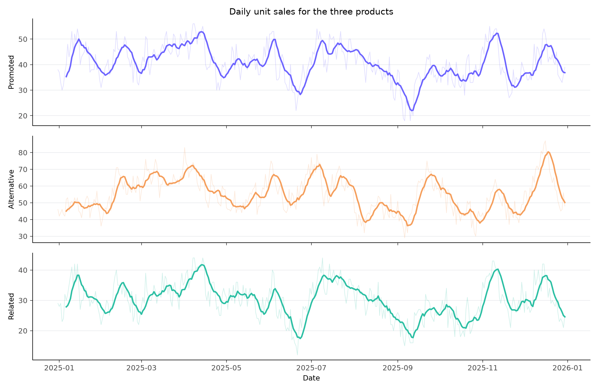 The three products share the same store, so they have busy days and quiet days
together — a rainy Saturday is slow for all of them. That shared movement is
real demand structure, and it is exactly what coupled simulation is built to
reproduce.
### Step 3: Define the Promotion
The next 28 days carry regular prices. Create a second plan with the promoted
product's price reduced by 15%, leaving the other prices unchanged:
```python theme={null}
promotion_X_df = current_X_df.copy()
promotion_X_df["promoted_price"] *= 0.85
```
### Step 4: Simulate the Product Group Under Both Plans
Generate 500 possible futures for all three products, first at current prices,
then with the promotion:
```python theme={null}
current_paths = nixtla_client.simulate(
df=df,
X_df=current_X_df,
h=h,
freq="D",
n_paths=500,
seed=42,
model="timegpt-2.1",
multivariate=True,
)
promotion_paths = nixtla_client.simulate(
df=df,
X_df=promotion_X_df,
h=h,
freq="D",
n_paths=500,
seed=42,
model="timegpt-2.1",
multivariate=True,
)
promotion_paths["coupled"].unique()
```
```text theme={null}
array([True])
```
The result confirms that the product paths were coupled. For example,
`sample_id=12` contains one 28-day future for each of the three products.
`multivariate=True` changes two things at once. TimeGPT 2.1 forecasts the
products jointly, so each product's forecast distribution can reflect the
others, and the sample paths are coupled, so one `sample_id` is one future for
the whole group. Both differences matter below.
### Step 5: Measure Lift, Cannibalization, and Cross-Selling
Product demand cannot be negative, so clip values at zero before calculating
unit totals:
```python theme={null}
def path_totals(paths):
nonnegative = paths.assign(
TimeGPT=paths["TimeGPT"].clip(lower=0)
)
return nonnegative.pivot_table(
index="sample_id",
columns="unique_id",
values="TimeGPT",
aggfunc="sum",
)
current_totals = path_totals(current_paths)
promotion_totals = path_totals(promotion_paths)
impact = pd.DataFrame(
{
"Current prices": current_totals.median(),
"Promotion": promotion_totals.median(),
}
)
impact["Change"] = impact["Promotion"] - impact["Current prices"]
impact["Change (%)"] = (
impact["Promotion"] / impact["Current prices"] - 1
)
impact
```
| unique\_id | Current prices | Promotion | Change | Change (%) |
| ------------------- | -------------: | --------: | -----: | ---------: |
| Alternative product | 1,526.8 | 1,347.8 | −179.0 | −11.7% |
| Promoted product | 1,102.3 | 1,167.8 | +65.5 | +6.0% |
| Related product | 788.1 | 830.6 | +42.5 | +5.4% |
The promoted product gains approximately 66 units. The related product gains
approximately 42 units — the cross-selling signal. The alternative product
loses approximately 179 units — the cannibalization signal. All three
directions match the relationships built into the data (the
[technical notes](#technical-notes) compare the sizes too).
This changes the business interpretation. Looking only at the promoted product
suggests a successful promotion. Looking at the complete product group shows that
the alternative product loses more units than the other two gain combined.
### Step 6: Estimate Shared-Demand Risk
To see what simulating the products *together* changes, generate the promotion
paths once more with the products simulated separately:
```python theme={null}
separate_paths = nixtla_client.simulate(
df=df,
X_df=promotion_X_df,
h=h,
freq="D",
n_paths=500,
seed=7,
model="timegpt-2.1",
multivariate=False,
)
separate_paths["coupled"].unique()
```
```text theme={null}
array([False])
```
The three products share the same store, so they have busy days and quiet days
together — a rainy Saturday is slow for all of them. That shared movement is
real demand structure, and it is exactly what coupled simulation is built to
reproduce.
### Step 3: Define the Promotion
The next 28 days carry regular prices. Create a second plan with the promoted
product's price reduced by 15%, leaving the other prices unchanged:
```python theme={null}
promotion_X_df = current_X_df.copy()
promotion_X_df["promoted_price"] *= 0.85
```
### Step 4: Simulate the Product Group Under Both Plans
Generate 500 possible futures for all three products, first at current prices,
then with the promotion:
```python theme={null}
current_paths = nixtla_client.simulate(
df=df,
X_df=current_X_df,
h=h,
freq="D",
n_paths=500,
seed=42,
model="timegpt-2.1",
multivariate=True,
)
promotion_paths = nixtla_client.simulate(
df=df,
X_df=promotion_X_df,
h=h,
freq="D",
n_paths=500,
seed=42,
model="timegpt-2.1",
multivariate=True,
)
promotion_paths["coupled"].unique()
```
```text theme={null}
array([True])
```
The result confirms that the product paths were coupled. For example,
`sample_id=12` contains one 28-day future for each of the three products.
`multivariate=True` changes two things at once. TimeGPT 2.1 forecasts the
products jointly, so each product's forecast distribution can reflect the
others, and the sample paths are coupled, so one `sample_id` is one future for
the whole group. Both differences matter below.
### Step 5: Measure Lift, Cannibalization, and Cross-Selling
Product demand cannot be negative, so clip values at zero before calculating
unit totals:
```python theme={null}
def path_totals(paths):
nonnegative = paths.assign(
TimeGPT=paths["TimeGPT"].clip(lower=0)
)
return nonnegative.pivot_table(
index="sample_id",
columns="unique_id",
values="TimeGPT",
aggfunc="sum",
)
current_totals = path_totals(current_paths)
promotion_totals = path_totals(promotion_paths)
impact = pd.DataFrame(
{
"Current prices": current_totals.median(),
"Promotion": promotion_totals.median(),
}
)
impact["Change"] = impact["Promotion"] - impact["Current prices"]
impact["Change (%)"] = (
impact["Promotion"] / impact["Current prices"] - 1
)
impact
```
| unique\_id | Current prices | Promotion | Change | Change (%) |
| ------------------- | -------------: | --------: | -----: | ---------: |
| Alternative product | 1,526.8 | 1,347.8 | −179.0 | −11.7% |
| Promoted product | 1,102.3 | 1,167.8 | +65.5 | +6.0% |
| Related product | 788.1 | 830.6 | +42.5 | +5.4% |
The promoted product gains approximately 66 units. The related product gains
approximately 42 units — the cross-selling signal. The alternative product
loses approximately 179 units — the cannibalization signal. All three
directions match the relationships built into the data (the
[technical notes](#technical-notes) compare the sizes too).
This changes the business interpretation. Looking only at the promoted product
suggests a successful promotion. Looking at the complete product group shows that
the alternative product loses more units than the other two gain combined.
### Step 6: Estimate Shared-Demand Risk
To see what simulating the products *together* changes, generate the promotion
paths once more with the products simulated separately:
```python theme={null}
separate_paths = nixtla_client.simulate(
df=df,
X_df=promotion_X_df,
h=h,
freq="D",
n_paths=500,
seed=7,
model="timegpt-2.1",
multivariate=False,
)
separate_paths["coupled"].unique()
```
```text theme={null}
array([False])
```
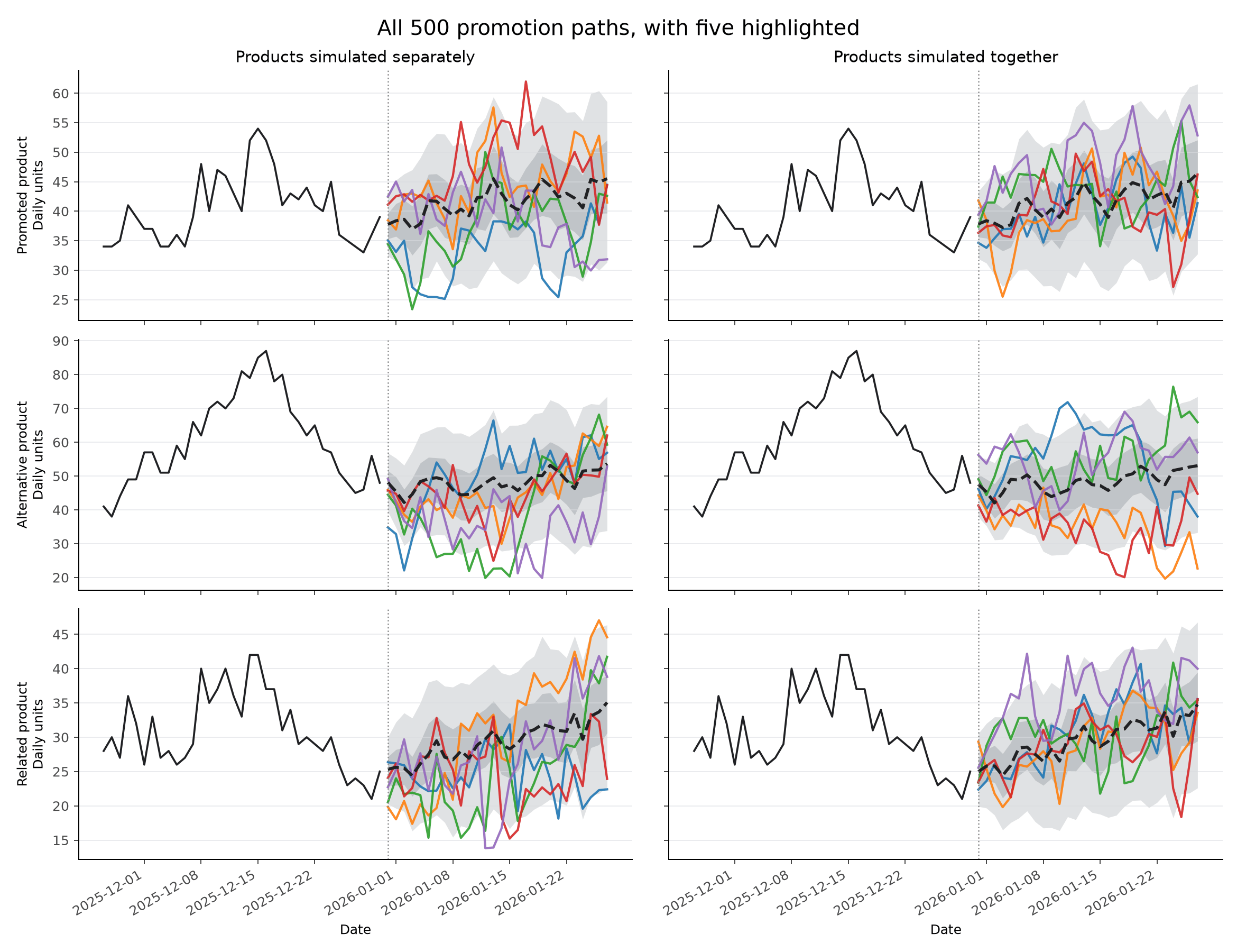 Follow one color down the right-hand column. The orange and red paths run low in
all three products, and the purple path runs high in all three: each color is one
future for the complete product group, and the store's busy and quiet days
reappear as products that are busy together. Down the left-hand column the same
colors do not line up — blue is among the lowest paths for the promoted product
and the highest for the alternative one — so no single path there describes the
group.
The two runs use different seeds on purpose. Reusing one seed can return
identical paths for the first product in both runs, which would make one row of
the chart above appear twice. The [technical notes](#technical-notes) explain
why.
Now ask an operational question:
> What is the chance that at least two products experience high demand on the
> same day during the promotion?
For this example, “high demand” means demand above that product's 90th
percentile in the separately simulated paths. The same thresholds are applied to
both sets of paths.
```python theme={null}
def daily_paths(paths):
nonnegative = paths.assign(
TimeGPT=paths["TimeGPT"].clip(lower=0)
)
return nonnegative.pivot(
index=["sample_id", "ds"],
columns="unique_id",
values="TimeGPT",
)
separate_daily = daily_paths(separate_paths)
coupled_daily = daily_paths(promotion_paths)
high_demand = separate_daily.quantile(0.90)
def simultaneous_high_demand(daily):
two_or_more = daily.gt(high_demand).sum(axis=1).ge(2)
return two_or_more.groupby("sample_id").any().mean()
separate_risk = simultaneous_high_demand(separate_daily)
coupled_risk = simultaneous_high_demand(coupled_daily)
separate_risk, coupled_risk
```
```text theme={null}
(0.424, 0.538)
```
Follow one color down the right-hand column. The orange and red paths run low in
all three products, and the purple path runs high in all three: each color is one
future for the complete product group, and the store's busy and quiet days
reappear as products that are busy together. Down the left-hand column the same
colors do not line up — blue is among the lowest paths for the promoted product
and the highest for the alternative one — so no single path there describes the
group.
The two runs use different seeds on purpose. Reusing one seed can return
identical paths for the first product in both runs, which would make one row of
the chart above appear twice. The [technical notes](#technical-notes) explain
why.
Now ask an operational question:
> What is the chance that at least two products experience high demand on the
> same day during the promotion?
For this example, “high demand” means demand above that product's 90th
percentile in the separately simulated paths. The same thresholds are applied to
both sets of paths.
```python theme={null}
def daily_paths(paths):
nonnegative = paths.assign(
TimeGPT=paths["TimeGPT"].clip(lower=0)
)
return nonnegative.pivot(
index=["sample_id", "ds"],
columns="unique_id",
values="TimeGPT",
)
separate_daily = daily_paths(separate_paths)
coupled_daily = daily_paths(promotion_paths)
high_demand = separate_daily.quantile(0.90)
def simultaneous_high_demand(daily):
two_or_more = daily.gt(high_demand).sum(axis=1).ge(2)
return two_or_more.groupby("sample_id").any().mean()
separate_risk = simultaneous_high_demand(separate_daily)
coupled_risk = simultaneous_high_demand(coupled_daily)
separate_risk, coupled_risk
```
```text theme={null}
(0.424, 0.538)
```
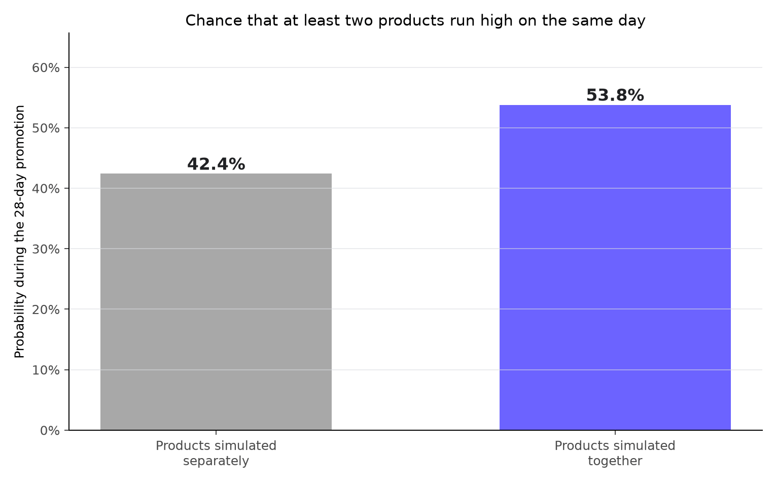 Simulating the products separately estimates a **42.4%** chance of simultaneous
high demand. Simulating them together raises that estimate to **53.8%**.
The products share a demand driver the model never sees. Simulating each one on
its own throws that shared movement away and treats busy days as independent
coincidences. Coupling puts it back, and more of the futures contain a day when
several products are under pressure at once.
Planning each product on its own understates how often they will need attention
at the same time. That 11.4-percentage-point gap can affect replenishment
staffing, shelf capacity, and safety-stock decisions.
## Turn the Result into a Retail Decision
This example suggests three actions:
1. Increase inventory for the promoted product.
2. Prepare for additional related-product demand.
3. Reduce the alternative product's order or reconsider the discount if total
product-group volume is the goal.
The final decision should include revenue, product margin, inventory cost, and
stockout cost. Those values can be calculated for every `sample_id`, producing a
distribution of profit instead of only a distribution of units.
With real sales data, a demand response like this is an association rather than
proof of a mechanism. Prices are usually set alongside promotions and seasonal
events, so a measured cross-product effect can reflect a shared calendar instead
of shoppers substituting. Use experiments or basket data when you need to
establish why customers changed their purchases.
## When Coupled Simulation Is Useful
Use coupled simulation when a decision combines several related series, such as:
* Ordering a family of substitute or complementary products
* Staffing a shared fulfillment operation
* Estimating total category revenue
* Planning capacity for products promoted at the same time
If each product is planned and fulfilled independently, ordinary simulation may
be sufficient. See [Simulation](/docs/forecasting/probabilistic/simulation) for the
complete API guide.
## Technical Notes
### The planted relationships
Calling one product a substitute and another a complement is only honest if
those relationships are actually in the data. Here they are written into the
generator, so the labels are true by construction and the simulation's answers
can be checked against them.
| Tutorial label | Planted role | Response to a 15% cut in the promoted price |
| ------------------- | -------------------------------------------------------------------- | ------------------------------------------: |
| Promoted product | Own-price elasticity | +11.9% |
| Alternative product | **Substitute** — loses demand when the promoted product gets cheaper | −11.5% |
| Related product | **Complement** — gains demand alongside the promoted product | +15.0% |
Two more properties matter:
* Each product has its **own price schedule**, and the three do not move
together. A promotion on one product is therefore a change the model can
attribute to that product.
* An **unobserved store-footfall factor** lifts all three products on the same
day. It is never passed to the model, so it survives as demand that moves
together across the products — which is exactly what coupling has to
reproduce. The products' demand rank correlations over the history are 0.49
between the promoted and alternative products, 0.88 between the promoted and
related products, and 0.47 between the alternative and related products.
### Recovered versus planted effects
Compare the simulated changes from Step 5 with the planted effects. The
cannibalization comes back almost exactly (−11.7% against a planted −11.5%),
while the two gains come back at roughly half their planted size (+6.0% against
+11.9%, and +5.4% against +15.0%). Forecasting a price level the model has not
seen is conservative by nature, so treat these as directionally right and, for
the gains, understated — not as exact elasticities.
### Why the seed differs between the coupled and separate runs
Both the coupled and the per-series shuffle draw their template windows from the
same random state, so with a fixed seed the first product by name is reordered
identically whether `multivariate` is True or False — for this data it comes
back with exactly the same 500 paths. Varying the seed removes this overlap
when the two runs are compared visually.
Simulating the products separately estimates a **42.4%** chance of simultaneous
high demand. Simulating them together raises that estimate to **53.8%**.
The products share a demand driver the model never sees. Simulating each one on
its own throws that shared movement away and treats busy days as independent
coincidences. Coupling puts it back, and more of the futures contain a day when
several products are under pressure at once.
Planning each product on its own understates how often they will need attention
at the same time. That 11.4-percentage-point gap can affect replenishment
staffing, shelf capacity, and safety-stock decisions.
## Turn the Result into a Retail Decision
This example suggests three actions:
1. Increase inventory for the promoted product.
2. Prepare for additional related-product demand.
3. Reduce the alternative product's order or reconsider the discount if total
product-group volume is the goal.
The final decision should include revenue, product margin, inventory cost, and
stockout cost. Those values can be calculated for every `sample_id`, producing a
distribution of profit instead of only a distribution of units.
With real sales data, a demand response like this is an association rather than
proof of a mechanism. Prices are usually set alongside promotions and seasonal
events, so a measured cross-product effect can reflect a shared calendar instead
of shoppers substituting. Use experiments or basket data when you need to
establish why customers changed their purchases.
## When Coupled Simulation Is Useful
Use coupled simulation when a decision combines several related series, such as:
* Ordering a family of substitute or complementary products
* Staffing a shared fulfillment operation
* Estimating total category revenue
* Planning capacity for products promoted at the same time
If each product is planned and fulfilled independently, ordinary simulation may
be sufficient. See [Simulation](/docs/forecasting/probabilistic/simulation) for the
complete API guide.
## Technical Notes
### The planted relationships
Calling one product a substitute and another a complement is only honest if
those relationships are actually in the data. Here they are written into the
generator, so the labels are true by construction and the simulation's answers
can be checked against them.
| Tutorial label | Planted role | Response to a 15% cut in the promoted price |
| ------------------- | -------------------------------------------------------------------- | ------------------------------------------: |
| Promoted product | Own-price elasticity | +11.9% |
| Alternative product | **Substitute** — loses demand when the promoted product gets cheaper | −11.5% |
| Related product | **Complement** — gains demand alongside the promoted product | +15.0% |
Two more properties matter:
* Each product has its **own price schedule**, and the three do not move
together. A promotion on one product is therefore a change the model can
attribute to that product.
* An **unobserved store-footfall factor** lifts all three products on the same
day. It is never passed to the model, so it survives as demand that moves
together across the products — which is exactly what coupling has to
reproduce. The products' demand rank correlations over the history are 0.49
between the promoted and alternative products, 0.88 between the promoted and
related products, and 0.47 between the alternative and related products.
### Recovered versus planted effects
Compare the simulated changes from Step 5 with the planted effects. The
cannibalization comes back almost exactly (−11.7% against a planted −11.5%),
while the two gains come back at roughly half their planted size (+6.0% against
+11.9%, and +5.4% against +15.0%). Forecasting a price level the model has not
seen is conservative by nature, so treat these as directionally right and, for
the gains, understated — not as exact elasticities.
### Why the seed differs between the coupled and separate runs
Both the coupled and the per-series shuffle draw their template windows from the
same random state, so with a fixed seed the first product by name is reordered
identically whether `multivariate` is True or False — for this data it comes
back with exactly the same 500 paths. Varying the seed removes this overlap
when the two runs are compared visually.