> ## Documentation Index
> Fetch the complete documentation index at: https://nixtla.io/docs/llms.txt
> Use this file to discover all available pages before exploring further.
# Hierarchical Forecasting
> Learn how to use TimeGPT for hierarchical forecasting across multiple levels.
## What is Hierarchical Forecasting?
Hierarchical forecasting involves generating forecasts for multiple time series that share a hierarchical structure (e.g., product demand by category, department, or region). The goal is to ensure that forecasts are coherent across each level of the hierarchy.
Hierarchical forecasting can be particularly important when you need to generate forecasts at different granularities (e.g., country, state, region) and ensure they align with each other and aggregate correctly at higher levels.
Using TimeGPT, you can create forecasts for multiple related time series and then apply hierarchical forecasting methods from [HierarchicalForecast](https://nixtlaverse.nixtla.io/hierarchicalforecast/index.html) to reconcile those forecasts across your specified hierarchy.
## Why use Hierarchical Forecasting?
* Ensures consistency: Forecasts at lower levels add up to higher-level forecasts.
* Improves accuracy: Reconciliation methods often yield more robust predictions.
* Facilitates deeper insights: Understand how smaller segments contribute to overall trends.
## Tutorial
[](https://colab.research.google.com/github/Nixtla/nixtla/blob/main/nbs/docs/tutorials/14_hierarchical_forecasting.ipynb)
### Step 1: Install, Import and Initialize
Start by installing the required packages.
```shell theme={null}
pip install nixtla
pip install hierarchicalforecast
```
Next, initialize the TimeGPT NixtlaClient.
```python theme={null}
import pandas as pd
import numpy as np
from nixtla import NixtlaClient
nixtla_client = NixtlaClient(
api_key='my_api_key_provided_by_nixtla'
)
```
### Step 2: Load and Prepare Data
This tutorial uses the Australian Tourism dataset from
[Forecasting: Principles and Practices](https://otexts.com/fpp3/). The dataset
contains different levels of hierarchical data, from the entire country of
Australia down to individual regions.

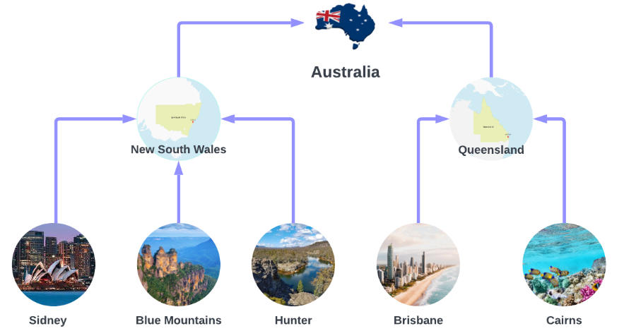 The dataset provides only the lowest-level series, so higher-level series need
to be aggregated explicitly. Let's load and preprocess the dataset.
```python theme={null}
Y_df = pd.read_csv(
'https://raw.githubusercontent.com/Nixtla/transfer-learning-time-series/main/datasets/tourism.csv'
)
Y_df = Y_df.rename({'Trips': 'y', 'Quarter': 'ds'}, axis=1)
Y_df.insert(0, 'Country', 'Australia')
Y_df = Y_df[['Country', 'Region', 'State', 'Purpose', 'ds', 'y']]
Y_df['ds'] = Y_df['ds'].str.replace(r'(\d+) (Q\d)', r'\1-\2', regex=True)
Y_df['ds'] = pd.to_datetime(Y_df['ds'])
Y_df.head(10)
```
| Country | Region | State | Purpose | ds | y |
| --------- | -------- | --------------- | -------- | ---------- | ---------- |
| Australia | Adelaide | South Australia | Business | 1998-01-01 | 135.077690 |
| Australia | Adelaide | South Australia | Business | 1998-04-01 | 109.987316 |
| Australia | Adelaide | South Australia | Business | 1998-07-01 | 166.034687 |
| Australia | Adelaide | South Australia | Business | 1998-10-01 | 127.160464 |
| Australia | Adelaide | South Australia | Business | 1999-01-01 | 137.448533 |
| Australia | Adelaide | South Australia | Business | 1999-04-01 | 199.912586 |
| Australia | Adelaide | South Australia | Business | 1999-07-01 | 169.355090 |
| Australia | Adelaide | South Australia | Business | 1999-10-01 | 134.357937 |
| Australia | Adelaide | South Australia | Business | 2000-01-01 | 154.034398 |
| Australia | Adelaide | South Australia | Business | 2000-04-01 | 168.776364 |
We define the dataset hierarchies explicitly. Each level in the list describes
one view of the hierarchy:
```python theme={null}
spec = [
['Country'],
['Country', 'State'],
['Country', 'Purpose'],
['Country', 'State', 'Region'],
['Country', 'State', 'Purpose'],
['Country', 'State', 'Region', 'Purpose']
]
```
Then, use `aggregate` from `HierarchicalForecast` to generate the aggregated series:
```python theme={null}
from hierarchicalforecast.utils import aggregate
Y_df, S_df, tags = aggregate(Y_df, spec)
Y_df.head(10)
```
| unique\_id | ds | y |
| ---------- | ---------- | ------------ |
| Australia | 1998-01-01 | 23182.197269 |
| Australia | 1998-04-01 | 20323.380067 |
| Australia | 1998-07-01 | 19826.640511 |
| Australia | 1998-10-01 | 20830.129891 |
| Australia | 1999-01-01 | 22087.353380 |
| Australia | 1999-04-01 | 21458.373285 |
| Australia | 1999-07-01 | 19914.192508 |
| Australia | 1999-10-01 | 20027.925640 |
| Australia | 2000-01-01 | 22339.294779 |
| Australia | 2000-04-01 | 19941.063482 |
Next, create the train/test splits. Here, we use the last two years (eight
quarters) of data for testing:
```python theme={null}
Y_test_df = Y_df.groupby('unique_id').tail(8)
Y_train_df = Y_df.drop(Y_test_df.index)
```
### Step 3: Hierarchical Forecasting Using TimeGPT
Now we'll generate base forecasts across all series using TimeGPT and then apply
hierarchical reconciliation to ensure the forecasts align across each level.
#### Generate Base Forecasts with TimeGPT
Obtain forecasts with TimeGPT for all series in your training data.
```python theme={null}
timegpt_fcst = nixtla_client.forecast(
df=Y_train_df,
h=8,
freq='QS',
add_history=True
)
```
Next, separate the generated forecasts into in-sample (historical) and
out-of-sample (forecasted) periods:
```python theme={null}
timegpt_fcst_insample = timegpt_fcst.query("ds < '2016-01-01'")
timegpt_fcst_outsample = timegpt_fcst.query("ds >= '2016-01-01'")
```
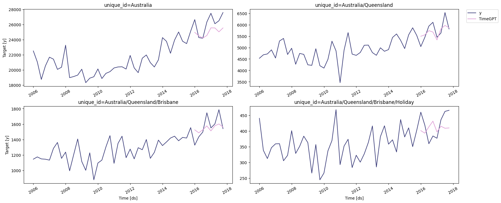
#### Visualize TimeGPT Forecasts
Quickly visualize the forecasts for different hierarchy levels. Here, we look at
the entire country, the state of Queensland, the Brisbane region, and holidays
in Brisbane:
```python theme={null}
nixtla_client.plot(
Y_df,
timegpt_fcst_outsample,
max_insample_length=4 * 12,
unique_ids=[
'Australia',
'Australia/Queensland',
'Australia/Queensland/Brisbane',
'Australia/Queensland/Brisbane/Holiday'
]
)
```
The dataset provides only the lowest-level series, so higher-level series need
to be aggregated explicitly. Let's load and preprocess the dataset.
```python theme={null}
Y_df = pd.read_csv(
'https://raw.githubusercontent.com/Nixtla/transfer-learning-time-series/main/datasets/tourism.csv'
)
Y_df = Y_df.rename({'Trips': 'y', 'Quarter': 'ds'}, axis=1)
Y_df.insert(0, 'Country', 'Australia')
Y_df = Y_df[['Country', 'Region', 'State', 'Purpose', 'ds', 'y']]
Y_df['ds'] = Y_df['ds'].str.replace(r'(\d+) (Q\d)', r'\1-\2', regex=True)
Y_df['ds'] = pd.to_datetime(Y_df['ds'])
Y_df.head(10)
```
| Country | Region | State | Purpose | ds | y |
| --------- | -------- | --------------- | -------- | ---------- | ---------- |
| Australia | Adelaide | South Australia | Business | 1998-01-01 | 135.077690 |
| Australia | Adelaide | South Australia | Business | 1998-04-01 | 109.987316 |
| Australia | Adelaide | South Australia | Business | 1998-07-01 | 166.034687 |
| Australia | Adelaide | South Australia | Business | 1998-10-01 | 127.160464 |
| Australia | Adelaide | South Australia | Business | 1999-01-01 | 137.448533 |
| Australia | Adelaide | South Australia | Business | 1999-04-01 | 199.912586 |
| Australia | Adelaide | South Australia | Business | 1999-07-01 | 169.355090 |
| Australia | Adelaide | South Australia | Business | 1999-10-01 | 134.357937 |
| Australia | Adelaide | South Australia | Business | 2000-01-01 | 154.034398 |
| Australia | Adelaide | South Australia | Business | 2000-04-01 | 168.776364 |
We define the dataset hierarchies explicitly. Each level in the list describes
one view of the hierarchy:
```python theme={null}
spec = [
['Country'],
['Country', 'State'],
['Country', 'Purpose'],
['Country', 'State', 'Region'],
['Country', 'State', 'Purpose'],
['Country', 'State', 'Region', 'Purpose']
]
```
Then, use `aggregate` from `HierarchicalForecast` to generate the aggregated series:
```python theme={null}
from hierarchicalforecast.utils import aggregate
Y_df, S_df, tags = aggregate(Y_df, spec)
Y_df.head(10)
```
| unique\_id | ds | y |
| ---------- | ---------- | ------------ |
| Australia | 1998-01-01 | 23182.197269 |
| Australia | 1998-04-01 | 20323.380067 |
| Australia | 1998-07-01 | 19826.640511 |
| Australia | 1998-10-01 | 20830.129891 |
| Australia | 1999-01-01 | 22087.353380 |
| Australia | 1999-04-01 | 21458.373285 |
| Australia | 1999-07-01 | 19914.192508 |
| Australia | 1999-10-01 | 20027.925640 |
| Australia | 2000-01-01 | 22339.294779 |
| Australia | 2000-04-01 | 19941.063482 |
Next, create the train/test splits. Here, we use the last two years (eight
quarters) of data for testing:
```python theme={null}
Y_test_df = Y_df.groupby('unique_id').tail(8)
Y_train_df = Y_df.drop(Y_test_df.index)
```
### Step 3: Hierarchical Forecasting Using TimeGPT
Now we'll generate base forecasts across all series using TimeGPT and then apply
hierarchical reconciliation to ensure the forecasts align across each level.
#### Generate Base Forecasts with TimeGPT
Obtain forecasts with TimeGPT for all series in your training data.
```python theme={null}
timegpt_fcst = nixtla_client.forecast(
df=Y_train_df,
h=8,
freq='QS',
add_history=True
)
```
Next, separate the generated forecasts into in-sample (historical) and
out-of-sample (forecasted) periods:
```python theme={null}
timegpt_fcst_insample = timegpt_fcst.query("ds < '2016-01-01'")
timegpt_fcst_outsample = timegpt_fcst.query("ds >= '2016-01-01'")
```
#### Visualize TimeGPT Forecasts
Quickly visualize the forecasts for different hierarchy levels. Here, we look at
the entire country, the state of Queensland, the Brisbane region, and holidays
in Brisbane:
```python theme={null}
nixtla_client.plot(
Y_df,
timegpt_fcst_outsample,
max_insample_length=4 * 12,
unique_ids=[
'Australia',
'Australia/Queensland',
'Australia/Queensland/Brisbane',
'Australia/Queensland/Brisbane/Holiday'
]
)
```
 #### Apply Hierarchical Reconciliation
We use `MinTrace` methods to reconcile forecasts across all levels of the hierarchy.
The `S` parameter was renamed to `S_df` in `hierarchicalforecast`. Make sure
you are using `S_df` when calling `reconcile`.
```python theme={null}
from hierarchicalforecast.methods import MinTrace
from hierarchicalforecast.core import HierarchicalReconciliation
reconcilers = [
MinTrace(method='ols'),
MinTrace(method='mint_shrink')
]
hrec = HierarchicalReconciliation(reconcilers=reconcilers)
Y_df_with_insample_fcsts = timegpt_fcst_insample.merge(Y_df.copy())
Y_rec_df = hrec.reconcile(
Y_hat_df=timegpt_fcst_outsample,
Y_df=Y_df_with_insample_fcsts,
S_df=S_df,
tags=tags
)
```
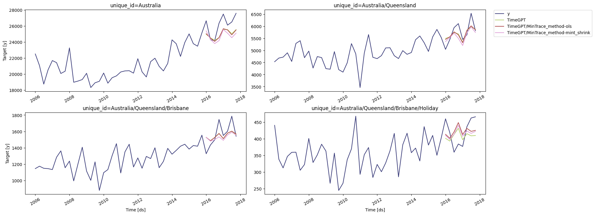
Now, let's plot the reconciled forecasts to ensure they make sense across the
full country → state → region → purpose hierarchy:
```python theme={null}
nixtla_client.plot(
Y_df,
Y_rec_df,
max_insample_length=4 * 12,
unique_ids=[
'Australia',
'Australia/Queensland',
'Australia/Queensland/Brisbane',
'Australia/Queensland/Brisbane/Holiday'
]
)
```
#### Apply Hierarchical Reconciliation
We use `MinTrace` methods to reconcile forecasts across all levels of the hierarchy.
The `S` parameter was renamed to `S_df` in `hierarchicalforecast`. Make sure
you are using `S_df` when calling `reconcile`.
```python theme={null}
from hierarchicalforecast.methods import MinTrace
from hierarchicalforecast.core import HierarchicalReconciliation
reconcilers = [
MinTrace(method='ols'),
MinTrace(method='mint_shrink')
]
hrec = HierarchicalReconciliation(reconcilers=reconcilers)
Y_df_with_insample_fcsts = timegpt_fcst_insample.merge(Y_df.copy())
Y_rec_df = hrec.reconcile(
Y_hat_df=timegpt_fcst_outsample,
Y_df=Y_df_with_insample_fcsts,
S_df=S_df,
tags=tags
)
```
Now, let's plot the reconciled forecasts to ensure they make sense across the
full country → state → region → purpose hierarchy:
```python theme={null}
nixtla_client.plot(
Y_df,
Y_rec_df,
max_insample_length=4 * 12,
unique_ids=[
'Australia',
'Australia/Queensland',
'Australia/Queensland/Brisbane',
'Australia/Queensland/Brisbane/Holiday'
]
)
```
 ### Step 4: Evaluate Forecast Accuracy
Finally, evaluate your forecast performance using RMSE for different levels of
the hierarchy, from total (country) to bottom-level (region/purpose).
```python theme={null}
from hierarchicalforecast.evaluation import evaluate
from utilsforecast.losses import rmse
eval_tags = {
'Total': tags['Country'],
'Purpose': tags['Country/Purpose'],
'State': tags['Country/State'],
'Regions': tags['Country/State/Region'],
'Bottom': tags['Country/State/Region/Purpose']
}
evaluation = evaluate(
df=Y_rec_df.merge(Y_test_df, on=['unique_id', 'ds']),
tags=eval_tags,
train_df=Y_train_df,
metrics=[rmse]
)
evaluation[evaluation.select_dtypes(np.number).columns] = evaluation.select_dtypes(np.number).map('{:.2f}'.format)
evaluation
```
| | level | metric | TimeGPT | TimeGPT/MinTrace\_method-ols | TimeGPT/MinTrace\_method-mint\_shrink |
| - | ------- | ------ | ------- | ---------------------------- | ------------------------------------- |
| 0 | Total | rmse | 1433.07 | 1436.07 | 1627.43 |
| 1 | Purpose | rmse | 482.09 | 475.64 | 507.50 |
| 2 | State | rmse | 275.85 | 278.39 | 294.28 |
| 3 | Regions | rmse | 49.40 | 47.91 | 47.99 |
| 4 | Bottom | rmse | 19.32 | 19.11 | 18.86 |
| 5 | Overall | rmse | 38.66 | 38.21 | 39.16 |
## Conclusion
We made a small improvement in overall RMSE by reconciling the forecasts with
`MinTrace(ols)`, and made them slightly worse using `MinTrace(mint_shrink)`,
indicating that the base forecasts were relatively strong already.
However, we now have coherent forecasts too - so not only did we make a (small)
accuracy improvement, we also got coherency to the hierarchy as a result of our
reconciliation step.
## References
* [Hyndman, Rob J., and George Athanasopoulos (2021). Forecasting: Principles and Practice](https://otexts.com/fpp3/).
### Step 4: Evaluate Forecast Accuracy
Finally, evaluate your forecast performance using RMSE for different levels of
the hierarchy, from total (country) to bottom-level (region/purpose).
```python theme={null}
from hierarchicalforecast.evaluation import evaluate
from utilsforecast.losses import rmse
eval_tags = {
'Total': tags['Country'],
'Purpose': tags['Country/Purpose'],
'State': tags['Country/State'],
'Regions': tags['Country/State/Region'],
'Bottom': tags['Country/State/Region/Purpose']
}
evaluation = evaluate(
df=Y_rec_df.merge(Y_test_df, on=['unique_id', 'ds']),
tags=eval_tags,
train_df=Y_train_df,
metrics=[rmse]
)
evaluation[evaluation.select_dtypes(np.number).columns] = evaluation.select_dtypes(np.number).map('{:.2f}'.format)
evaluation
```
| | level | metric | TimeGPT | TimeGPT/MinTrace\_method-ols | TimeGPT/MinTrace\_method-mint\_shrink |
| - | ------- | ------ | ------- | ---------------------------- | ------------------------------------- |
| 0 | Total | rmse | 1433.07 | 1436.07 | 1627.43 |
| 1 | Purpose | rmse | 482.09 | 475.64 | 507.50 |
| 2 | State | rmse | 275.85 | 278.39 | 294.28 |
| 3 | Regions | rmse | 49.40 | 47.91 | 47.99 |
| 4 | Bottom | rmse | 19.32 | 19.11 | 18.86 |
| 5 | Overall | rmse | 38.66 | 38.21 | 39.16 |
## Conclusion
We made a small improvement in overall RMSE by reconciling the forecasts with
`MinTrace(ols)`, and made them slightly worse using `MinTrace(mint_shrink)`,
indicating that the base forecasts were relatively strong already.
However, we now have coherent forecasts too - so not only did we make a (small)
accuracy improvement, we also got coherency to the hierarchy as a result of our
reconciliation step.
## References
* [Hyndman, Rob J., and George Athanasopoulos (2021). Forecasting: Principles and Practice](https://otexts.com/fpp3/).