> ## Documentation Index
> Fetch the complete documentation index at: https://nixtla.io/docs/llms.txt
> Use this file to discover all available pages before exploring further.

# Test forecast sensitivity

> See how a TimeGPT forecast changes when one input is replaced by its typical historical value.

Use an intervention explanation when someone asks:

> Which inputs could meaningfully change this forecast?

TimeGPT replaces one input at a time with its typical historical value and runs
the forecast again. The difference shows how sensitive the model is to that
input.

## Retail-demand example

We use the same store example as the [SHAP
guide](/docs/forecasting/exogenous-variables/interpretability_with_shap): 365 days of
demand, price, promotion, and temperature, followed by a 14-day forecast.

<Accordion title="Create the example data">
  ```python theme={null}
  import numpy as np
  import pandas as pd

  from nixtla import NixtlaClient

  nixtla_client = NixtlaClient(
      # Defaults to os.environ["NIXTLA_API_KEY"]
      api_key="my_api_key_provided_by_nixtla"
  )

  rng = np.random.default_rng(7)
  n = 365
  h = 14
  t = np.arange(n + h)

  price = 20 + 1.8 * np.sin(2 * np.pi * t / 90) + rng.normal(0, 0.35, n + h)
  promotion = ((t % 42) >= 35).astype(int)
  temperature = (
      18
      + 9 * np.sin(2 * np.pi * (t - 30) / 365)
      + rng.normal(0, 0.8, n + h)
  )
  weekly = 6 * np.sin(2 * np.pi * t / 7)
  demand = (
      118
      - 2.4 * price[:n]
      + 16 * promotion[:n]
      + 0.55 * temperature[:n]
      + weekly[:n]
      + rng.normal(0, 2.0, n)
  )

  dates = pd.date_range("2024-01-01", periods=n + h, freq="D")
  df = pd.DataFrame(
      {
          "unique_id": "store-a",
          "ds": dates[:n],
          "y": demand,
          "price": price[:n],
          "promotion": promotion[:n],
          "temperature": temperature[:n],
      }
  )
  X_df = pd.DataFrame(
      {
          "unique_id": "store-a",
          "ds": dates[n:],
          "price": price[n:],
          "promotion": promotion[n:],
          "temperature": temperature[n:],
      }
  )
  ```
</Accordion>

## Run the sensitivity analysis

Select the intervention explanation when making the forecast:

```python theme={null}
forecast = nixtla_client.forecast(
    df=df,
    X_df=X_df,
    h=h,
    freq="D",
    model="timegpt-2.1",
    feature_contributions=True,
    feature_contributions_type="intervention",
)

sensitivity = nixtla_client.feature_contributions
```

For numerical inputs, TimeGPT uses the historical average as the typical value.
For categorical inputs, it uses the most common historical value.

<Warning>
  Intervention shows how the **model** responds when an input is replaced, which doesn't necessarily translate to how the real world would respond. Treat it as a starting point for investigation, not a causal estimate.
</Warning>

## Summarize the promotion period

The future data contains a seven-day promotion. Average the sensitivity values
over those days:

```python theme={null}
features = ["price", "promotion", "temperature"]
promotion_dates = X_df.loc[X_df["promotion"].eq(1), "ds"]

promotion_sensitivity = sensitivity.loc[
    sensitivity["ds"].isin(promotion_dates),
    features,
].mean()

promotion_sensitivity
```

| Input       | Average forecast difference |
| ----------- | --------------------------: |
| Price       |                 -1.00 units |
| Promotion   |                 +1.00 units |
| Temperature |                 -0.63 units |

During the promotion period:

* The observed promotion raises the model forecast by about **one unit**
  compared with a typical promotion value.
* The observed price lowers it by about **one unit** compared with the store's
  historical average price.
* The observed temperature lowers it by about **0.63 units** compared with the
  historical average temperature.

## See how sensitivity changes by day

<Frame caption="Each line shows the difference between the observed-input forecast and the forecast with that input set to its typical value. Results were generated with TimeGPT 2.1.">
  <img src="https://mintcdn.com/nixtla-enterprise/Z27JIqRDnQ0rRCKY/images/forecasting/explain-retail-intervention.png?fit=max&auto=format&n=Z27JIqRDnQ0rRCKY&q=85&s=bd34276e772c655990a6c41af675bbe5" alt="A line chart showing daily forecast sensitivity to price, promotion, and temperature" width="1961" height="915" data-path="images/forecasting/explain-retail-intervention.png" />
</Frame>

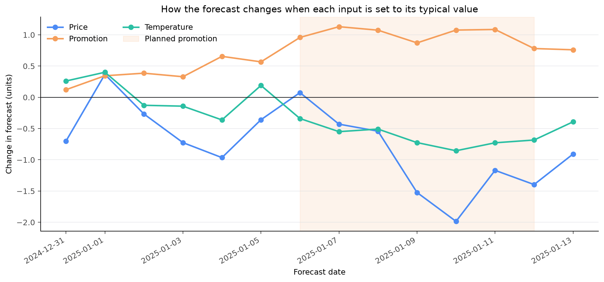The model's sensitivity is not constant. Price has a larger effect on some days,
while promotion stays positive throughout the planned promotion period. This is
why the daily result is often more useful than a single overall average.

## When to use intervention

Intervention explanations are helpful when:

* A forecast changes after new price, weather, or campaign information arrives.
* You want to compare the model forecast with a familiar historical reference.
* You need to identify forecast inputs worth reviewing with a domain expert.

## Next

* [Explain a forecast with
  SHAP](/docs/forecasting/exogenous-variables/interpretability_with_shap)
* [Find predictive signals in
  history](/docs/forecasting/exogenous-variables/causal-explanations)
* [Advanced explanations](/docs/forecasting/explanation/advanced-explanations)