> ## Documentation Index
> Fetch the complete documentation index at: https://nixtla.io/docs/llms.txt
> Use this file to discover all available pages before exploring further.
# Numeric Variables
> Learn how to incorporate external numeric variables to improve your forecasting accuracy.
## What Are Exogenous Variables?
Exogenous variables or external factors are crucial in time series forecasting
as they provide additional information that might influence the prediction.
These variables could include holiday markers, marketing spending, weather data,
or any other external data that correlate with the time series data you are
forecasting.
For example, if you're forecasting ice cream sales, temperature data could serve
as a useful exogenous variable. On hotter days, ice cream sales may increase.
## How to Use Exogenous Variables
[](https://colab.research.google.com/github/Nixtla/nixtla/blob/main/nbs/docs/tutorials/01_exogenous_variables_reworked.ipynb)
To incorporate exogenous variables in TimeGPT, you'll need to pair each point
in your time series data with the corresponding external data.
### Step 1: Import Packages
Import the required libraries and initialize the Nixtla client.
```python theme={null}
import pandas as pd
from nixtla import NixtlaClient
nixtla_client = NixtlaClient(
# defaults to os.environ.get("NIXTLA_API_KEY")
api_key="my_api_key_provided_by_nixtla"
)
```
### Step 2: Load Dataset
In this tutorial, we'll predict day-ahead electricity prices. The dataset contains:
* Hourly electricity prices (`y`) from various markets (identified by `unique_id`)
* Exogenous variables (`Exogenous1` to `day_6`)
```python theme={null}
df = pd.read_csv("https://raw.githubusercontent.com/Nixtla/transfer-learning-time-series/main/datasets/electricity-short-with-ex-vars.csv")
df.head()
```
| unique\_id | ds | y | Exogenous1 | Exogenous2 | day\_0 | day\_1 | day\_2 | day\_3 | day\_4 | day\_5 | day\_6 |
| ---------- | ------------------- | ----- | ---------- | ---------- | ------ | ------ | ------ | ------ | ------ | ------ | ------ |
| BE | 2016-10-22 00:00:00 | 70.00 | 57253.0 | 49593.0 | 0.0 | 0.0 | 0.0 | 0.0 | 0.0 | 1.0 | 0.0 |
| BE | 2016-10-22 01:00:00 | 37.10 | 51887.0 | 46073.0 | 0.0 | 0.0 | 0.0 | 0.0 | 0.0 | 1.0 | 0.0 |
| BE | 2016-10-22 02:00:00 | 37.10 | 51896.0 | 44927.0 | 0.0 | 0.0 | 0.0 | 0.0 | 0.0 | 1.0 | 0.0 |
| BE | 2016-10-22 03:00:00 | 44.75 | 48428.0 | 44483.0 | 0.0 | 0.0 | 0.0 | 0.0 | 0.0 | 1.0 | 0.0 |
| BE | 2016-10-22 04:00:00 | 37.10 | 46721.0 | 44338.0 | 0.0 | 0.0 | 0.0 | 0.0 | 0.0 | 1.0 | 0.0 |
### Step 3: Forecast without Exogenous Variables
First, let's create a baseline forecast without using any exogenous variables.
```python theme={null}
timegpt_fcst_no_ex_vars = nixtla_client.forecast(
df=df[["unique_id", "ds", "y"]],
h=24,
level=[80, 90]
)
```
### Step 4: Forecasting with Exogenous Variables
Next, let's create a forecast using the exogenous variables. To make a forecast
using exogenous variables, you need to provide historical and future exogenous
values. Below is an example dataset containing future exogenous variables. Note
that it only contains the future exogenous variable values not the target
variable `y`. We need to forecast this target variable using the exogenous
variables provided.
```python theme={null}
future_ex_vars_df = pd.read_csv("https://raw.githubusercontent.com/Nixtla/transfer-learning-time-series/main/datasets/electricity-short-future-ex-vars.csv")
future_ex_vars_df.head()
```
| unique\_id | ds | Exogenous1 | Exogenous2 | day\_0 | day\_1 | day\_2 | day\_3 | day\_4 | day\_5 | day\_6 |
| ---------- | ------------------- | ---------- | ---------- | ------ | ------ | ------ | ------ | ------ | ------ | ------ |
| BE | 2016-12-31 00:00:00 | 70318.0 | 64108.0 | 0.0 | 0.0 | 0.0 | 0.0 | 0.0 | 1.0 | 0.0 |
| BE | 2016-12-31 01:00:00 | 67898.0 | 62492.0 | 0.0 | 0.0 | 0.0 | 0.0 | 0.0 | 1.0 | 0.0 |
| BE | 2016-12-31 02:00:00 | 68379.0 | 61571.0 | 0.0 | 0.0 | 0.0 | 0.0 | 0.0 | 1.0 | 0.0 |
| BE | 2016-12-31 03:00:00 | 64972.0 | 60381.0 | 0.0 | 0.0 | 0.0 | 0.0 | 0.0 | 1.0 | 0.0 |
| BE | 2016-12-31 04:00:00 | 62900.0 | 60298.0 | 0.0 | 0.0 | 0.0 | 0.0 | 0.0 | 1.0 | 0.0 |
Ensure you maintain consistent data formatting and columns in both historical
and future exogenous datasets (e.g., dates, unique\_id, variable names).
```python theme={null}
timegpt_fcst_ex_vars = nixtla_client.forecast(
df=df,
X_df=future_ex_vars_df,
h=24,
level=[80, 90]
)
```
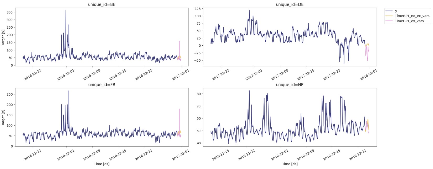
### Step 5: Forecast Visualization
Once you have generated your forecasts, you can visualize the results to compare
forecasts between the two methods above.
```python theme={null}
timegpt_fcst_no_ex_vars.rename(columns={"TimeGPT": "TimeGPT_no_ex_vars"}, inplace=True)
timegpt_fcst_ex_vars.rename(columns={"TimeGPT": "TimeGPT_ex_vars"}, inplace=True)
all_forecasts = (
timegpt_fcst_no_ex_vars
.merge(
timegpt_fcst_ex_vars,
how='outer',
on=["unique_id", "ds"]
)
)
```
```python theme={null}
nixtla_client.plot(
df[["unique_id", "ds", "y"]],
all_forecasts,
max_insample_length=1000,
)
```
 ## Key Takeaways
* Exogenous variables enrich time series forecasting.
* Ensure proper alignment of historical and future exogenous data.
## Next Steps
Congratulations! You have mastered the fundamentals of adding exogenous
variables to your TimeGPT forecasts. Keep refining your approach by
* Exploring feature engineering to create domain-specific exogenous data.
* Experimenting with different modeling approaches for external variables.
* Validating forecast accuracy by comparing with real future data.
## Key Takeaways
* Exogenous variables enrich time series forecasting.
* Ensure proper alignment of historical and future exogenous data.
## Next Steps
Congratulations! You have mastered the fundamentals of adding exogenous
variables to your TimeGPT forecasts. Keep refining your approach by
* Exploring feature engineering to create domain-specific exogenous data.
* Experimenting with different modeling approaches for external variables.
* Validating forecast accuracy by comparing with real future data.