> ## Documentation Index
> Fetch the complete documentation index at: https://nixtla.io/docs/llms.txt
> Use this file to discover all available pages before exploring further.
# Find predictive signals in history
> Rank the features that have been most useful for predicting your target over time.
Use `NixtlaClient.explain()` when someone asks:
> Which signals in my historical data deserve attention?
The result ranks your features using their past relationship with the target.
You do not need to make a forecast or provide future feature values.
The analysis runs as an asynchronous job on the server. `NixtlaClient.explain()`
submits the job and polls its status until the weights are ready, so the call
blocks like any other client method. By default the client waits up to 10
minutes; adjust `async_job_wait_timeout` and `async_job_poll_interval` when
creating the `NixtlaClient` if you need a different behavior. A job that fails
on the server raises `nixtla.AsyncJobError` with the server's original error. Server-side cancellation raises
`nixtla.AsyncJobCancelledError`; exceeding the client wait timeout raises
`nixtla.AsyncJobTimeoutError` and requests cancellation.
These weights are **not** causal. They measure whether a feature's past values
help predict the target, which is a statement about correlation over time, not
about cause and effect. A high weight does not mean that changing the feature
will change the target: both may be driven by something absent from your data,
or the direction of influence may run the other way. To ask what a forecast is
sensitive to, use [intervention
analysis](/docs/forecasting/explanation/intervention) instead.
## Retail-demand example
The store in our example has one year of daily demand, price, promotion, and
temperature data.
```python theme={null}
import numpy as np
import pandas as pd
from nixtla import NixtlaClient
nixtla_client = NixtlaClient(
# Defaults to os.environ["NIXTLA_API_KEY"]
api_key="my_api_key_provided_by_nixtla"
)
rng = np.random.default_rng(7)
n = 365
h = 14
t = np.arange(n + h)
price = 20 + 1.8 * np.sin(2 * np.pi * t / 90) + rng.normal(0, 0.35, n + h)
promotion = ((t % 42) >= 35).astype(int)
temperature = (
18
+ 9 * np.sin(2 * np.pi * (t - 30) / 365)
+ rng.normal(0, 0.8, n + h)
)
weekly = 6 * np.sin(2 * np.pi * t / 7)
demand = (
118
- 2.4 * price[:n]
+ 16 * promotion[:n]
+ 0.55 * temperature[:n]
+ weekly[:n]
+ rng.normal(0, 2.0, n)
)
df = pd.DataFrame(
{
"unique_id": "store-a",
"ds": pd.date_range("2024-01-01", periods=n, freq="D"),
"y": demand,
"price": price[:n],
"promotion": promotion[:n],
"temperature": temperature[:n],
}
)
```
## Rank the historical signals
Call `explain()` with the features you want to review:
```python theme={null}
signals = nixtla_client.explain(
df=df,
features=["price", "promotion", "temperature"],
)
signals
```
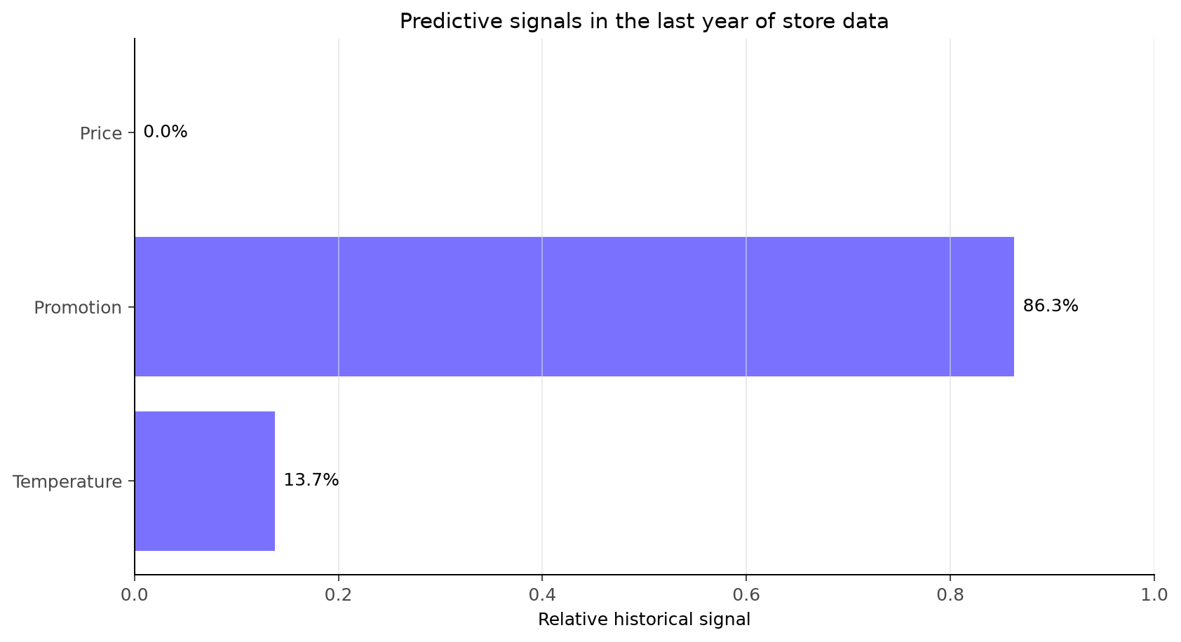
| feature | weight | method |
| ----------- | -----: | ------- |
| price | 0.000 | granger |
| promotion | 0.863 | granger |
| temperature | 0.137 | granger |
The weights add up to one. In this historical window, promotion has the
strongest measured signal, followed by temperature. Price does not add a
measurable linear lagged signal in this particular run.
 ## Use the ranking
This result can help you:
* Decide which data sources deserve closer monitoring.
* Prioritize features for a forecasting experiment.
* Check whether important business signals are present in the data.
* Compare feature rankings across stores, products, or time periods.
It cannot tell you what to change. "Promotion ranks first, so running more
promotions will raise demand" does not follow from this ranking; it is a causal
claim the analysis does not support.
Weights are relative scores. A weight of `0.863` means promotion is the
strongest signal among these three features; it is not a percentage of the
forecast.
## Use your own data
By default, `explain()` analyzes every column except the series ID, timestamp,
and target. Passing `features` makes the scope explicit:
```python theme={null}
signals = nixtla_client.explain(
df=df,
features=["price", "promotion", "temperature"],
)
```
For multiple time series, stack the series in the same dataframe and identify
them with `unique_id`. TimeGPT respects the boundary between each series and
returns one combined ranking.
Non-numeric features must be declared as categorical. Any feature that is not
numeric and not listed in `categorical_exog_list` is rejected, naming the
column:
```python theme={null}
df_with_campaign = df.assign(
campaign=np.where(df["promotion"] == 1, "email", "none")
)
signals = nixtla_client.explain(
df=df_with_campaign,
features=["price", "promotion", "temperature", "campaign"],
categorical_exog_list=["campaign"],
)
```
Both methods are lag-based, so every series must be complete and regularly
spaced. `explain()` infers the frequency from `df`; pass `freq` explicitly for
polars input, or to be strict about which spacing you expect:
```python theme={null}
signals = nixtla_client.explain(df=df, freq="D")
```
Historical signals are especially useful for exploration and feature
prioritization. Re-run an important analysis on another time period to see
whether the same signals remain useful.
## Next
* [Explain a forecast with
SHAP](/docs/forecasting/exogenous-variables/interpretability_with_shap)
* [Test forecast sensitivity](/docs/forecasting/explanation/intervention)
* [Compare analyses and check
stability](/docs/forecasting/explanation/advanced-explanations)
## Use the ranking
This result can help you:
* Decide which data sources deserve closer monitoring.
* Prioritize features for a forecasting experiment.
* Check whether important business signals are present in the data.
* Compare feature rankings across stores, products, or time periods.
It cannot tell you what to change. "Promotion ranks first, so running more
promotions will raise demand" does not follow from this ranking; it is a causal
claim the analysis does not support.
Weights are relative scores. A weight of `0.863` means promotion is the
strongest signal among these three features; it is not a percentage of the
forecast.
## Use your own data
By default, `explain()` analyzes every column except the series ID, timestamp,
and target. Passing `features` makes the scope explicit:
```python theme={null}
signals = nixtla_client.explain(
df=df,
features=["price", "promotion", "temperature"],
)
```
For multiple time series, stack the series in the same dataframe and identify
them with `unique_id`. TimeGPT respects the boundary between each series and
returns one combined ranking.
Non-numeric features must be declared as categorical. Any feature that is not
numeric and not listed in `categorical_exog_list` is rejected, naming the
column:
```python theme={null}
df_with_campaign = df.assign(
campaign=np.where(df["promotion"] == 1, "email", "none")
)
signals = nixtla_client.explain(
df=df_with_campaign,
features=["price", "promotion", "temperature", "campaign"],
categorical_exog_list=["campaign"],
)
```
Both methods are lag-based, so every series must be complete and regularly
spaced. `explain()` infers the frequency from `df`; pass `freq` explicitly for
polars input, or to be strict about which spacing you expect:
```python theme={null}
signals = nixtla_client.explain(df=df, freq="D")
```
Historical signals are especially useful for exploration and feature
prioritization. Re-run an important analysis on another time period to see
whether the same signals remain useful.
## Next
* [Explain a forecast with
SHAP](/docs/forecasting/exogenous-variables/interpretability_with_shap)
* [Test forecast sensitivity](/docs/forecasting/explanation/intervention)
* [Compare analyses and check
stability](/docs/forecasting/explanation/advanced-explanations)