> ## Documentation Index
> Fetch the complete documentation index at: https://nixtla.io/docs/llms.txt
> Use this file to discover all available pages before exploring further.
# Categorical Variables
> Learn how to incorporate external categorical variables in your TimeGPT forecasts to improve accuracy.
## What Are Categorical Variables?
Categorical variables are external factors that take on a limited range of discrete values, grouping observations by categories. For example, "Sporting" or "Cultural" events in a dataset describing product demand.
By capturing unique external conditions, categorical variables enhance the predictive power of your model and can reduce forecasting error. They are easy to incorporate by merging each time series data point with its corresponding categorical data.
This tutorial demonstrates how to incorporate categorical (discrete) variables into TimeGPT forecasts.
## How to Use Categorical Variables in TimeGPT
[](https://colab.research.google.com/github/Nixtla/nixtla/blob/main/nbs/docs/tutorials/03_categorical_variables.ipynb)
### Step 1: Import Packages and Initialize the Nixtla Client
Make sure you have the necessary libraries installed: pandas, nixtla, and datasetsforecast.
```python theme={null}
import pandas as pd
import os
from nixtla import NixtlaClient
from datasetsforecast.m5 import M5
from utilsforecast.losses import smape
# Initialize the Nixtla Client
nixtla_client = NixtlaClient(
api_key='my_api_key_provided_by_nixtla'
)
```
### Step 2: Load M5 Data
We use the **M5 dataset** — a collection of daily product sales demands across 10 US stores — to showcase how categorical variables can improve forecasts.
Start by loading the M5 dataset and converting the date columns to datetime objects.
```python theme={null}
Y_df, X_df, _ = M5.load(directory=os.getcwd())
Y_df['ds'] = pd.to_datetime(Y_df['ds'])
X_df['ds'] = pd.to_datetime(X_df['ds'])
Y_df.head(10)
```
| unique\_id | ds | y |
| -------------------- | ---------- | --- |
| FOODS\_1\_001\_CA\_1 | 2011-01-29 | 3.0 |
| FOODS\_1\_001\_CA\_1 | 2011-01-30 | 0.0 |
| FOODS\_1\_001\_CA\_1 | 2011-01-31 | 0.0 |
| FOODS\_1\_001\_CA\_1 | 2011-02-01 | 1.0 |
| FOODS\_1\_001\_CA\_1 | 2011-02-02 | 4.0 |
| FOODS\_1\_001\_CA\_1 | 2011-02-03 | 2.0 |
| FOODS\_1\_001\_CA\_1 | 2011-02-04 | 0.0 |
| FOODS\_1\_001\_CA\_1 | 2011-02-05 | 2.0 |
| FOODS\_1\_001\_CA\_1 | 2011-02-06 | 0.0 |
| FOODS\_1\_001\_CA\_1 | 2011-02-07 | 0.0 |
Extract the categorical columns from the X\_df dataframe.
```python theme={null}
X_df = X_df[['unique_id', 'ds', 'event_type_1']]
X_df.head(10)
```
| unique\_id | ds | event\_type\_1 |
| -------------------- | ---------- | -------------- |
| FOODS\_1\_001\_CA\_1 | 2011-01-29 | nan |
| FOODS\_1\_001\_CA\_1 | 2011-01-30 | nan |
| FOODS\_1\_001\_CA\_1 | 2011-01-31 | nan |
| FOODS\_1\_001\_CA\_1 | 2011-02-01 | nan |
| FOODS\_1\_001\_CA\_1 | 2011-02-02 | nan |
| FOODS\_1\_001\_CA\_1 | 2011-02-03 | nan |
| FOODS\_1\_001\_CA\_1 | 2011-02-04 | nan |
| FOODS\_1\_001\_CA\_1 | 2011-02-05 | nan |
| FOODS\_1\_001\_CA\_1 | 2011-02-06 | Sporting |
| FOODS\_1\_001\_CA\_1 | 2011-02-07 | nan |
Notice that there is a Sporting event on February 6, 2011, listed under `event_type_1`.
### Step 3: Prepare Data for Forecasting
We'll select a specific product to demonstrate how to incorporate categorical features into TimeGPT forecasts.
#### Select a High-Selling Product and Merge Data
Start by selecting a high-selling product and merging the data.
```python theme={null}
product = 'FOODS_3_090_CA_3'
Y_df_product = Y_df.query('unique_id == @product')
X_df_product = X_df.query('unique_id == @product')
df = Y_df_product.merge(X_df_product)
df.head(10)
```
| unique\_id | ds | y | event\_type\_1 |
| -------------------- | ---------- | ----- | -------------- |
| FOODS\_3\_090\_CA\_3 | 2011-01-29 | 108.0 | nan |
| FOODS\_3\_090\_CA\_3 | 2011-01-30 | 132.0 | nan |
| FOODS\_3\_090\_CA\_3 | 2011-01-31 | 102.0 | nan |
| FOODS\_3\_090\_CA\_3 | 2011-02-01 | 120.0 | nan |
| FOODS\_3\_090\_CA\_3 | 2011-02-02 | 106.0 | nan |
| FOODS\_3\_090\_CA\_3 | 2011-02-03 | 123.0 | nan |
| FOODS\_3\_090\_CA\_3 | 2011-02-04 | 279.0 | nan |
| FOODS\_3\_090\_CA\_3 | 2011-02-05 | 175.0 | nan |
| FOODS\_3\_090\_CA\_3 | 2011-02-06 | 186.0 | Sporting |
| FOODS\_3\_090\_CA\_3 | 2011-02-07 | 120.0 | nan |
#### Prepare Future External Variables
Select future external variables for Feb 1-7, 2016.
```python theme={null}
future_ex_vars_df = df.drop(columns=['y']).query("ds >= '2016-02-01' & ds <= '2016-02-07'")
```
Separate training data before Feb 1, 2016.
```python theme={null}
df_train = df.query("ds < '2016-02-01'")
df_train.tail(10)
```
| unique\_id | ds | y | event\_type\_1 |
| -------------------- | ---------- | ----- | -------------- |
| FOODS\_3\_090\_CA\_3 | 2016-01-22 | 94.0 | nan |
| FOODS\_3\_090\_CA\_3 | 2016-01-23 | 144.0 | nan |
| FOODS\_3\_090\_CA\_3 | 2016-01-24 | 146.0 | nan |
| FOODS\_3\_090\_CA\_3 | 2016-01-25 | 87.0 | nan |
| FOODS\_3\_090\_CA\_3 | 2016-01-26 | 73.0 | nan |
| FOODS\_3\_090\_CA\_3 | 2016-01-27 | 62.0 | nan |
| FOODS\_3\_090\_CA\_3 | 2016-01-28 | 64.0 | nan |
| FOODS\_3\_090\_CA\_3 | 2016-01-29 | 102.0 | nan |
| FOODS\_3\_090\_CA\_3 | 2016-01-30 | 113.0 | nan |
| FOODS\_3\_090\_CA\_3 | 2016-01-31 | 98.0 | nan |
### Step 4: Forecast Product Demand
To evaluate the impact of categorical variables, we'll forecast product demand with and without them.
#### Forecast Without Categorical Variables
```python theme={null}
timegpt_fcst_without_cat_vars_df = nixtla_client.forecast(
df=df_train,
h=7,
level=[80, 90]
)
timegpt_fcst_without_cat_vars_df.head()
```
| unique\_id | ds | TimeGPT | TimeGPT-hi-80 | TimeGPT-hi-90 | TimeGPT-lo-80 | TimeGPT-lo-90 |
| -------------------- | ---------- | --------- | ------------- | ------------- | ------------- | ------------- |
| FOODS\_3\_090\_CA\_3 | 2016-02-01 | 73.304090 | 95.887380 | 98.250880 | 50.720802 | 48.357307 |
| FOODS\_3\_090\_CA\_3 | 2016-02-02 | 66.335520 | 75.429660 | 76.663704 | 57.241375 | 56.007330 |
| FOODS\_3\_090\_CA\_3 | 2016-02-03 | 65.881630 | 86.636480 | 87.502810 | 45.126778 | 44.260456 |
| FOODS\_3\_090\_CA\_3 | 2016-02-04 | 72.371864 | 92.362690 | 96.378610 | 52.381035 | 48.365116 |
| FOODS\_3\_090\_CA\_3 | 2016-02-05 | 95.141045 | 111.439224 | 114.115490 | 78.842865 | 76.166595 |
Visualize the forecast without categorical variables.
```python theme={null}
nixtla_client.plot(
df[['unique_id', 'ds', 'y']].query("ds <= '2016-02-07'"),
timegpt_fcst_without_cat_vars_df,
max_insample_length=28,
)
```
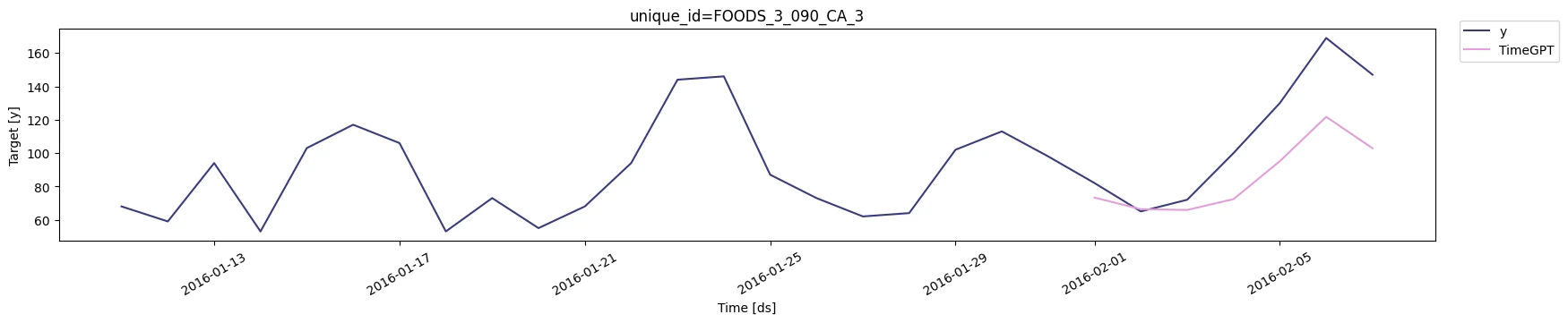 TimeGPT already provides a reasonable forecast, but it seems to somewhat underforecast the peak on the 6th of February 2016 - the day before the Super Bowl.
#### Forecast With Categorical Variables
To forecast with categorical variables, simply provide the list of column names containing categorical features in the `categorical_exog_list` argument.
```python theme={null}
timegpt_fcst_with_cat_vars_df = nixtla_client.forecast(
df=df_train,
X_df=future_ex_vars_df,
h=7,
level=[80, 90],
categorical_exog_list=["event_type_1"]
)
timegpt_fcst_with_cat_vars_df.head()
```
| unique\_id | ds | TimeGPT | TimeGPT-hi-80 | TimeGPT-hi-90 | TimeGPT-lo-80 | TimeGPT-lo-90 |
| -------------------- | ---------- | --------- | ------------- | ------------- | ------------- | ------------- |
| FOODS\_3\_090\_CA\_3 | 2016-02-01 | 73.839455 | 100.905910 | 104.44151 | 46.773006 | 43.237396 |
| FOODS\_3\_090\_CA\_3 | 2016-02-02 | 66.548750 | 75.294970 | 76.62822 | 57.802540 | 56.469284 |
| FOODS\_3\_090\_CA\_3 | 2016-02-03 | 66.694435 | 87.777954 | 88.63922 | 45.610912 | 44.749650 |
| FOODS\_3\_090\_CA\_3 | 2016-02-04 | 74.249530 | 94.813286 | 98.88473 | 53.685770 | 49.614326 |
| FOODS\_3\_090\_CA\_3 | 2016-02-05 | 96.052414 | 112.402090 | 115.22341 | 79.702736 | 76.881420 |
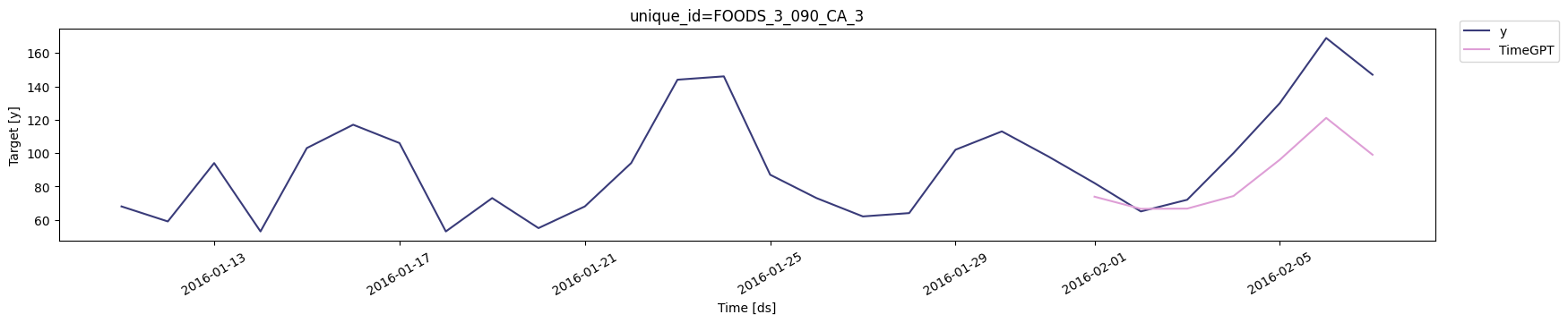
Visualize the forecast with categorical variables.
```python theme={null}
# Visualize the forecast with categorical variables
nixtla_client.plot(
df[['unique_id', 'ds', 'y']].query("ds <= '2016-02-07'"),
timegpt_fcst_with_cat_vars_df,
max_insample_length=28,
)
```
TimeGPT already provides a reasonable forecast, but it seems to somewhat underforecast the peak on the 6th of February 2016 - the day before the Super Bowl.
#### Forecast With Categorical Variables
To forecast with categorical variables, simply provide the list of column names containing categorical features in the `categorical_exog_list` argument.
```python theme={null}
timegpt_fcst_with_cat_vars_df = nixtla_client.forecast(
df=df_train,
X_df=future_ex_vars_df,
h=7,
level=[80, 90],
categorical_exog_list=["event_type_1"]
)
timegpt_fcst_with_cat_vars_df.head()
```
| unique\_id | ds | TimeGPT | TimeGPT-hi-80 | TimeGPT-hi-90 | TimeGPT-lo-80 | TimeGPT-lo-90 |
| -------------------- | ---------- | --------- | ------------- | ------------- | ------------- | ------------- |
| FOODS\_3\_090\_CA\_3 | 2016-02-01 | 73.839455 | 100.905910 | 104.44151 | 46.773006 | 43.237396 |
| FOODS\_3\_090\_CA\_3 | 2016-02-02 | 66.548750 | 75.294970 | 76.62822 | 57.802540 | 56.469284 |
| FOODS\_3\_090\_CA\_3 | 2016-02-03 | 66.694435 | 87.777954 | 88.63922 | 45.610912 | 44.749650 |
| FOODS\_3\_090\_CA\_3 | 2016-02-04 | 74.249530 | 94.813286 | 98.88473 | 53.685770 | 49.614326 |
| FOODS\_3\_090\_CA\_3 | 2016-02-05 | 96.052414 | 112.402090 | 115.22341 | 79.702736 | 76.881420 |
Visualize the forecast with categorical variables.
```python theme={null}
# Visualize the forecast with categorical variables
nixtla_client.plot(
df[['unique_id', 'ds', 'y']].query("ds <= '2016-02-07'"),
timegpt_fcst_with_cat_vars_df,
max_insample_length=28,
)
```
 ## 5. Evaluate Forecast Accuracy
Finally, we calculate the **Symmetric Mean Absolute Percentage Error (sMAPE)** for the forecasts with and without categorical variables.
```python theme={null}
# Create target dataframe
df_target = df[['unique_id', 'ds', 'y']].query("ds >= '2016-02-01' & ds <= '2016-02-07'")
# Rename forecast columns
timegpt_fcst_without_cat_vars_df = timegpt_fcst_without_cat_vars_df.rename(columns={'TimeGPT': 'TimeGPT-without-cat-vars'})
timegpt_fcst_with_cat_vars_df = timegpt_fcst_with_cat_vars_df.rename(columns={'TimeGPT': 'TimeGPT-with-cat-vars'})
# Merge forecasts with target dataframe
df_target = df_target.merge(timegpt_fcst_without_cat_vars_df[['unique_id', 'ds', 'TimeGPT-without-cat-vars']])
df_target = df_target.merge(timegpt_fcst_with_cat_vars_df[['unique_id', 'ds', 'TimeGPT-with-cat-vars']])
# Compute errors
smape_errors = smape(df_target, ['TimeGPT-without-cat-vars', 'TimeGPT-with-cat-vars'])
```
| unique\_id | TimeGPT-without-cat-vars | TimeGPT-with-cat-vars |
| -------------------- | ------------------------ | --------------------- |
| FOODS\_3\_090\_CA\_3 | 0.109241 | 0.108666 |
Including categorical variables improves forecast accuracy as it achieves a lower sMAPE.
## Conclusion
Categorical variables are powerful additions to TimeGPT forecasts, helping capture valuable external factors. By simply passing them to the `categorical_exog_list` parameter, you can significantly enhance predictive performance.
Continue exploring more advanced techniques or different datasets to further improve your TimeGPT forecasting models.
## 5. Evaluate Forecast Accuracy
Finally, we calculate the **Symmetric Mean Absolute Percentage Error (sMAPE)** for the forecasts with and without categorical variables.
```python theme={null}
# Create target dataframe
df_target = df[['unique_id', 'ds', 'y']].query("ds >= '2016-02-01' & ds <= '2016-02-07'")
# Rename forecast columns
timegpt_fcst_without_cat_vars_df = timegpt_fcst_without_cat_vars_df.rename(columns={'TimeGPT': 'TimeGPT-without-cat-vars'})
timegpt_fcst_with_cat_vars_df = timegpt_fcst_with_cat_vars_df.rename(columns={'TimeGPT': 'TimeGPT-with-cat-vars'})
# Merge forecasts with target dataframe
df_target = df_target.merge(timegpt_fcst_without_cat_vars_df[['unique_id', 'ds', 'TimeGPT-without-cat-vars']])
df_target = df_target.merge(timegpt_fcst_with_cat_vars_df[['unique_id', 'ds', 'TimeGPT-with-cat-vars']])
# Compute errors
smape_errors = smape(df_target, ['TimeGPT-without-cat-vars', 'TimeGPT-with-cat-vars'])
```
| unique\_id | TimeGPT-without-cat-vars | TimeGPT-with-cat-vars |
| -------------------- | ------------------------ | --------------------- |
| FOODS\_3\_090\_CA\_3 | 0.109241 | 0.108666 |
Including categorical variables improves forecast accuracy as it achieves a lower sMAPE.
## Conclusion
Categorical variables are powerful additions to TimeGPT forecasts, helping capture valuable external factors. By simply passing them to the `categorical_exog_list` parameter, you can significantly enhance predictive performance.
Continue exploring more advanced techniques or different datasets to further improve your TimeGPT forecasting models.